Computations and Masks with Xarray


Overview

In this tutorial, we will cover the following topics:

  1. Performing basic arithmetic on DataArrays and Datasets

  2. Performing aggregation (i.e., reduction) along single or multiple dimensions of a DataArray or Dataset

  3. Computing climatologies and anomalies of data using Xarray’s “split-apply-combine” approach, via the .groupby() method

  4. Performing weighted-reduction operations along single or multiple dimensions of a DataArray or Dataset

  5. Providing a broad overview of Xarray’s data-masking capability

  6. Using the .where() method to mask Xarray data

Prerequisites

Concepts

Importance

Notes

Introduction to Xarray

Necessary

  • Time to learn: 60 minutes


Imports

In order to work with data and plotting, we must import NumPy, Matplotlib, and Xarray. These packages are covered in greater detail in earlier tutorials. We also import a package that allows quick download of Pythia example datasets.

import matplotlib.pyplot as plt
import numpy as np
import xarray as xr
from pythia_datasets import DATASETS

Data Setup

The bulk of the examples in this tutorial make use of a single dataset. This dataset contains monthly sea surface temperature (SST, call ‘tos’ here) data, and is obtained from the Community Earth System Model v2 (CESM2). (For this tutorial, however, the dataset will be retrieved from the Pythia example data repository.) The following example illustrates the process of retrieving this Global Climate Model dataset:

filepath = DATASETS.fetch('CESM2_sst_data.nc')
ds = xr.open_dataset(filepath)
ds
Downloading file 'CESM2_sst_data.nc' from 'https://github.com/ProjectPythia/pythia-datasets/raw/main/data/CESM2_sst_data.nc' to '/home/runner/.cache/pythia-datasets'.
/home/runner/miniconda3/envs/pythia-book-dev/lib/python3.12/site-packages/xarray/conventions.py:286: SerializationWarning: variable 'tos' has multiple fill values {1e+20, 1e+20} defined, decoding all values to NaN.
  var = coder.decode(var, name=name)
<xarray.Dataset> Size: 47MB
Dimensions:    (time: 180, d2: 2, lat: 180, lon: 360)
Coordinates:
  * time       (time) object 1kB 2000-01-15 12:00:00 ... 2014-12-15 12:00:00
  * lat        (lat) float64 1kB -89.5 -88.5 -87.5 -86.5 ... 86.5 87.5 88.5 89.5
  * lon        (lon) float64 3kB 0.5 1.5 2.5 3.5 4.5 ... 356.5 357.5 358.5 359.5
Dimensions without coordinates: d2
Data variables:
    time_bnds  (time, d2) object 3kB ...
    lat_bnds   (lat, d2) float64 3kB ...
    lon_bnds   (lon, d2) float64 6kB ...
    tos        (time, lat, lon) float32 47MB ...
Attributes: (12/45)
    Conventions:            CF-1.7 CMIP-6.2
    activity_id:            CMIP
    branch_method:          standard
    branch_time_in_child:   674885.0
    branch_time_in_parent:  219000.0
    case_id:                972
    ...                     ...
    sub_experiment_id:      none
    table_id:               Omon
    tracking_id:            hdl:21.14100/2975ffd3-1d7b-47e3-961a-33f212ea4eb2
    variable_id:            tos
    variant_info:           CMIP6 20th century experiments (1850-2014) with C...
    variant_label:          r11i1p1f1

Arithmetic Operations

In a similar fashion to NumPy arrays, performing an arithmetic operation on a DataArray will automatically perform the operation on all array values; this is known as vectorization. To illustrate the process of vectorization, the following example converts the air temperature data from units of degrees Celsius to units of Kelvin:

ds.tos + 273.15
<xarray.DataArray 'tos' (time: 180, lat: 180, lon: 360)> Size: 47MB
array([[[      nan,       nan,       nan, ...,       nan,       nan,
               nan],
        [      nan,       nan,       nan, ...,       nan,       nan,
               nan],
        [      nan,       nan,       nan, ...,       nan,       nan,
               nan],
        ...,
        [271.3552 , 271.3553 , 271.3554 , ..., 271.35495, 271.355  ,
         271.3551 ],
        [271.36005, 271.36014, 271.36023, ..., 271.35986, 271.35992,
         271.36   ],
        [271.36447, 271.36453, 271.3646 , ..., 271.3643 , 271.36435,
         271.3644 ]],

       [[      nan,       nan,       nan, ...,       nan,       nan,
               nan],
        [      nan,       nan,       nan, ...,       nan,       nan,
               nan],
        [      nan,       nan,       nan, ...,       nan,       nan,
               nan],
...
        [271.40677, 271.40674, 271.4067 , ..., 271.40695, 271.4069 ,
         271.40683],
        [271.41296, 271.41293, 271.41293, ..., 271.41306, 271.413  ,
         271.41296],
        [271.41772, 271.41772, 271.41772, ..., 271.41766, 271.4177 ,
         271.4177 ]],

       [[      nan,       nan,       nan, ...,       nan,       nan,
               nan],
        [      nan,       nan,       nan, ...,       nan,       nan,
               nan],
        [      nan,       nan,       nan, ...,       nan,       nan,
               nan],
        ...,
        [271.39386, 271.39383, 271.3938 , ..., 271.39407, 271.394  ,
         271.39392],
        [271.39935, 271.39932, 271.39932, ..., 271.39948, 271.39944,
         271.39938],
        [271.40372, 271.40372, 271.40375, ..., 271.4037 , 271.4037 ,
         271.40372]]], dtype=float32)
Coordinates:
  * time     (time) object 1kB 2000-01-15 12:00:00 ... 2014-12-15 12:00:00
  * lat      (lat) float64 1kB -89.5 -88.5 -87.5 -86.5 ... 86.5 87.5 88.5 89.5
  * lon      (lon) float64 3kB 0.5 1.5 2.5 3.5 4.5 ... 356.5 357.5 358.5 359.5

In addition, there are many other arithmetic operations that can be performed on DataArrays. In this example, we demonstrate squaring the original Celsius values of our air temperature data:

ds.tos**2
<xarray.DataArray 'tos' (time: 180, lat: 180, lon: 360)> Size: 47MB
array([[[      nan,       nan,       nan, ...,       nan,       nan,
               nan],
        [      nan,       nan,       nan, ...,       nan,       nan,
               nan],
        [      nan,       nan,       nan, ...,       nan,       nan,
               nan],
        ...,
        [3.2213385, 3.2209656, 3.220537 , ..., 3.2221622, 3.221913 ,
         3.2216525],
        [3.203904 , 3.203617 , 3.2032912, ..., 3.2045207, 3.2043478,
         3.2041442],
        [3.1881146, 3.1879027, 3.1876712, ..., 3.188714 , 3.1885312,
         3.1883302]],

       [[      nan,       nan,       nan, ...,       nan,       nan,
               nan],
        [      nan,       nan,       nan, ...,       nan,       nan,
               nan],
        [      nan,       nan,       nan, ...,       nan,       nan,
               nan],
...
        [3.0388296, 3.0389647, 3.0390673, ..., 3.038165 , 3.0383828,
         3.0386322],
        [3.0173173, 3.0173445, 3.0173297, ..., 3.0169601, 3.0171173,
         3.0172386],
        [3.000791 , 3.0007784, 3.0007539, ..., 3.000933 , 3.000896 ,
         3.0008452]],

       [[      nan,       nan,       nan, ...,       nan,       nan,
               nan],
        [      nan,       nan,       nan, ...,       nan,       nan,
               nan],
        [      nan,       nan,       nan, ...,       nan,       nan,
               nan],
        ...,
        [3.0839543, 3.0841148, 3.0842566, ..., 3.0832636, 3.0834875,
         3.0837412],
        [3.064733 , 3.0648024, 3.0648358, ..., 3.0642793, 3.0644639,
         3.0646174],
        [3.0494578, 3.0494475, 3.0494263, ..., 3.049596 , 3.0495603,
         3.0495107]]], dtype=float32)
Coordinates:
  * time     (time) object 1kB 2000-01-15 12:00:00 ... 2014-12-15 12:00:00
  * lat      (lat) float64 1kB -89.5 -88.5 -87.5 -86.5 ... 86.5 87.5 88.5 89.5
  * lon      (lon) float64 3kB 0.5 1.5 2.5 3.5 4.5 ... 356.5 357.5 358.5 359.5

Aggregation Methods

A common practice in the field of data analysis is aggregation. Aggregation is the process of reducing data through methods such as sum(), mean(), median(), min(), and max(), in order to gain greater insight into the nature of large datasets. In this set of examples, we demonstrate correct usage of a select group of aggregation methods:

Compute the mean:

ds.tos.mean()
<xarray.DataArray 'tos' ()> Size: 4B
array(14.250171, dtype=float32)

Notice that we did not specify the dim keyword argument; this means that the function was applied over all of the dataset’s dimensions. In other words, the aggregation method computed the mean of every element of the temperature dataset across every temporal and spatial data point. However, if a dimension name is used with the dim keyword argument, the aggregation method computes an aggregation along the given dimension. In this next example, we use aggregation to calculate the temporal mean across all spatial data; this is performed by providing the dimension name 'time' to the dim keyword argument:

ds.tos.mean(dim='time').plot(size=7);
../../_images/cff85267ac822235de65b62d030988c5120d7670de42cf0e19b196cd17e9b95d.png

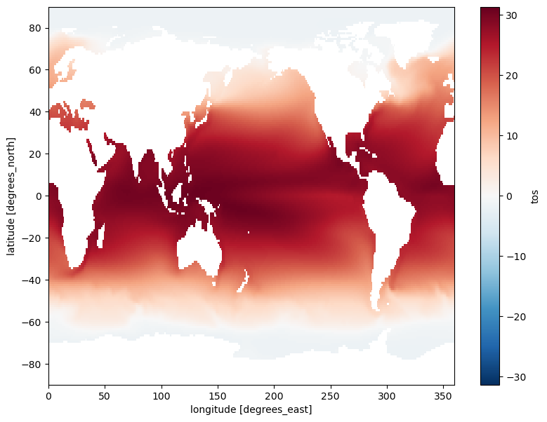
There are many other combinations of aggregation methods and dimensions on which to perform these methods. In this example, we compute the temporal minimum:

ds.tos.min(dim=['time'])
<xarray.DataArray 'tos' (lat: 180, lon: 360)> Size: 259kB
array([[       nan,        nan,        nan, ...,        nan,        nan,
               nan],
       [       nan,        nan,        nan, ...,        nan,        nan,
               nan],
       [       nan,        nan,        nan, ...,        nan,        nan,
               nan],
       ...,
       [-1.8083605, -1.8083031, -1.8082187, ..., -1.8083988, -1.8083944,
        -1.8083915],
       [-1.8025414, -1.8024837, -1.8024155, ..., -1.8026428, -1.8026177,
        -1.8025846],
       [-1.7984415, -1.7983989, -1.7983514, ..., -1.7985678, -1.7985296,
        -1.7984871]], dtype=float32)
Coordinates:
  * lat      (lat) float64 1kB -89.5 -88.5 -87.5 -86.5 ... 86.5 87.5 88.5 89.5
  * lon      (lon) float64 3kB 0.5 1.5 2.5 3.5 4.5 ... 356.5 357.5 358.5 359.5

This example computes the spatial sum. Note that this dataset contains no altitude data; as such, the required spatial dimensions passed to the method consist only of latitude and longitude.

ds.tos.sum(dim=['lat', 'lon'])
<xarray.DataArray 'tos' (time: 180)> Size: 720B
array([603767.  , 607702.5 , 603976.5 , 599373.56, 595119.94, 595716.75,
       598177.3 , 600670.6 , 597825.56, 591869.  , 590507.7 , 597189.2 ,
       605954.06, 609151.  , 606868.9 , 602329.9 , 599465.75, 601205.5 ,
       605144.4 , 608588.5 , 604046.9 , 598927.75, 597519.75, 603876.9 ,
       612424.44, 615765.2 , 612615.44, 606310.6 , 602034.4 , 600784.9 ,
       602013.5 , 603142.2 , 598850.9 , 591917.44, 589234.56, 596162.5 ,
       602942.06, 607196.9 , 604928.2 , 601735.6 , 599011.8 , 599490.9 ,
       600801.44, 602786.94, 598867.2 , 594081.8 , 593736.25, 598995.6 ,
       607285.25, 611901.06, 609562.75, 603527.3 , 600215.4 , 601372.6 ,
       604144.5 , 605376.75, 601256.2 , 595245.2 , 594002.06, 600490.4 ,
       611878.6 , 616563.  , 613050.8 , 605734.  , 600808.75, 600898.06,
       603930.56, 605644.7 , 599917.5 , 592048.06, 590082.8 , 596950.7 ,
       607701.94, 610844.7 , 609509.6 , 603380.94, 599838.1 , 600334.25,
       604386.6 , 607848.1 , 602155.2 , 594949.06, 593815.06, 598365.3 ,
       608730.8 , 612056.5 , 609922.5 , 603077.1 , 600134.1 , 602821.2 ,
       606152.75, 610257.8 , 604685.8 , 596858.  , 592894.8 , 599944.9 ,
       609764.44, 614610.75, 611434.75, 605606.4 , 603790.94, 605750.2 ,
       609250.06, 612935.7 , 609645.06, 601706.4 , 598896.5 , 605349.75,
       614671.8 , 618686.7 , 615895.2 , 609438.2 , 605399.56, 606126.75,
       607942.3 , 609680.4 , 604814.25, 595841.94, 591908.44, 595638.7 ,
       604798.94, 611327.1 , 609765.7 , 603727.56, 600970.  , 602514.  ,
       606303.7 , 609225.25, 603724.3 , 595944.8 , 594477.4 , 597807.4 ,
       607379.06, 611808.56, 610112.94, 607196.3 , 604733.06, 605488.25,
       610048.3 , 612655.75, 608906.25, 602349.7 , 601754.2 , 609220.4 ,
       619367.1 , 623783.2 , 619949.7 , 613369.06, 610190.8 , 611091.2 ,
       614213.44, 615665.06, 611722.2 , 606259.56, 605970.2 , 611463.3 ,
       619794.6 , 626036.5 , 623085.44, 616295.9 , 611886.3 , 611881.9 ,
       614420.75, 616853.56, 610375.44, 603471.5 , 602108.25, 608094.3 ,
       617450.7 , 623508.7 , 619830.2 , 612033.3 , 608737.2 , 610105.25,
       613692.7 , 616360.44, 611735.4 , 606512.7 , 604249.44, 608777.44],
      dtype=float32)
Coordinates:
  * time     (time) object 1kB 2000-01-15 12:00:00 ... 2014-12-15 12:00:00

For the last example in this set of aggregation examples, we compute the temporal median:

ds.tos.median(dim='time')
<xarray.DataArray 'tos' (lat: 180, lon: 360)> Size: 259kB
array([[       nan,        nan,        nan, ...,        nan,        nan,
               nan],
       [       nan,        nan,        nan, ...,        nan,        nan,
               nan],
       [       nan,        nan,        nan, ...,        nan,        nan,
               nan],
       ...,
       [-1.7648907, -1.7648032, -1.7647004, ..., -1.7650614, -1.7650102,
        -1.7649589],
       [-1.7590305, -1.7589546, -1.7588665, ..., -1.7591925, -1.7591486,
        -1.759095 ],
       [-1.7536805, -1.753602 , -1.7535168, ..., -1.753901 , -1.753833 ,
        -1.7537591]], dtype=float32)
Coordinates:
  * lat      (lat) float64 1kB -89.5 -88.5 -87.5 -86.5 ... 86.5 87.5 88.5 89.5
  * lon      (lon) float64 3kB 0.5 1.5 2.5 3.5 4.5 ... 356.5 357.5 358.5 359.5

In addition, there are many other commonly used aggregation methods in Xarray. Some of the more popular aggregation methods are summarized in the following table:

Aggregation

Description

count()

Total number of items

mean(), median()

Mean and median

min(), max()

Minimum and maximum

std(), var()

Standard deviation and variance

prod()

Compute product of elements

sum()

Compute sum of elements

argmin(), argmax()

Find index of minimum and maximum value

GroupBy: Split, Apply, Combine

While we can obtain useful summaries of datasets using simple aggregation methods, it is more often the case that aggregation must be performed over coordinate labels or groups. In order to perform this type of aggregation, it is helpful to use the split-apply-combine workflow. Fortunately, Xarray provides this functionality for DataArrays and Datasets by means of the groupby operation. The following figure illustrates the split-apply-combine workflow in detail:

../../_images/xarray-split-apply-combine.jpeg

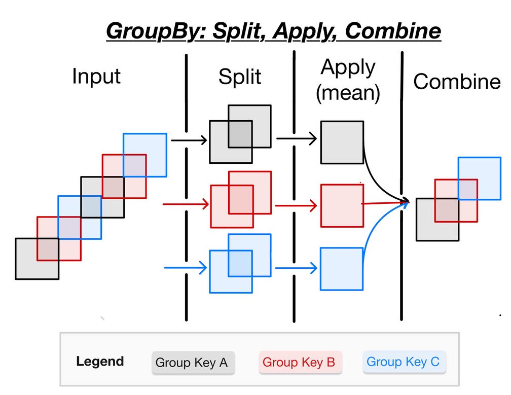
Based on the above figure, you can understand the split-apply-combine process performed by groupby. In detail, the steps of this process are:

  • The split step involves breaking up and grouping an xarray Dataset or DataArray depending on the value of the specified group key.

  • The apply step involves computing some function, usually an aggregate, transformation, or filtering, within the individual groups.

  • The combine step merges the results of these operations into an output xarray Dataset or DataArray.

In this set of examples, we will remove the seasonal cycle (also known as a climatology) from our dataset using groupby. There are many types of input that can be provided to groupby; a full list can be found in Xarray’s groupby user guide.

In this first example, we plot data to illustrate the annual cycle described above. We first select the grid point closest to a specific latitude-longitude point. Once we have this grid point, we can plot a temporal series of sea-surface temperature (SST) data at that location. Reviewing the generated plot, the annual cycle of the data becomes clear.

ds.tos.sel(lon=310, lat=50, method='nearest').plot();
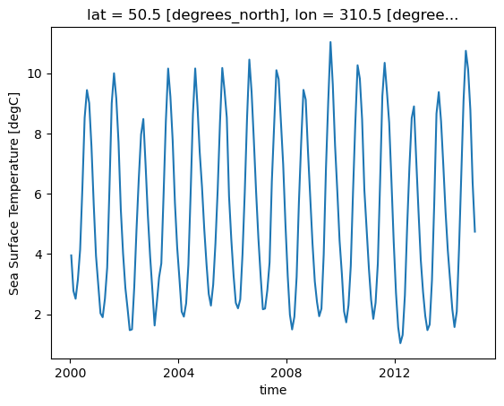
../../_images/f98b90b6eccc24379d8362dfabd794860f1c92c1998078ba525a9e0874d7d542.png

Split

The first step of the split-apply-combine process is splitting. As described above, this step involves splitting a dataset into groups, with each group matching a group key. In this example, we split the SST data using months as a group key. Therefore, there is one resulting group for January data, one for February data, etc. This code illustrates how to perform such a split:

ds.tos.groupby(ds.time.dt.month)
DataArrayGroupBy, grouped over 'month'
12 groups with labels 1, 2, 3, 4, 5, 6, 7, 8, 9, 10, 11, 12.

In the above code example, we are extracting components of date/time data by way of the time coordinate’s .dt attribute. This attribute is a DatetimeAccessor object that contains additional attributes for units of time, such as hour, day, and year. Since we are splitting the data into monthly data, we use the month attribute of .dt in this example. (In addition, there exists similar functionality in Pandas; see the official documentation for details.)

In addition, there is a more concise syntax that can be used in specific instances. This syntax can be used if the variable on which the grouping is performed is already present in the dataset. The following example illustrates this syntax; it is functionally equivalent to the syntax used in the above example.

ds.tos.groupby('time.month')
DataArrayGroupBy, grouped over 'month'
12 groups with labels 1, 2, 3, 4, 5, 6, 7, 8, 9, 10, 11, 12.

Apply & Combine

Now that we have split our data into groups, the next step is to apply a calculation to the groups. There are two types of calculation that can be applied:

  • aggregation: reduces the size of the group

  • transformation: preserves the group’s full size

After a calculation is applied to the groups, Xarray will automatically combine the groups back into a single object, completing the split-apply-combine workflow.

Compute climatology

In this example, we use the split-apply-combine workflow to calculate the monthly climatology at every point in the dataset. Notice that we are using the month DatetimeAccessor, as described above, as well as the .mean() aggregation function:

tos_clim = ds.tos.groupby('time.month').mean()
tos_clim
<xarray.DataArray 'tos' (month: 12, lat: 180, lon: 360)> Size: 3MB
array([[[       nan,        nan,        nan, ...,        nan,
                nan,        nan],
        [       nan,        nan,        nan, ...,        nan,
                nan,        nan],
        [       nan,        nan,        nan, ...,        nan,
                nan,        nan],
        ...,
        [-1.780786 , -1.780688 , -1.7805718, ..., -1.7809757,
         -1.7809197, -1.7808627],
        [-1.7745041, -1.7744204, -1.7743237, ..., -1.77467  ,
         -1.774626 , -1.7745715],
        [-1.7691481, -1.7690798, -1.7690051, ..., -1.7693441,
         -1.7692844, -1.7692182]],

       [[       nan,        nan,        nan, ...,        nan,
                nan,        nan],
        [       nan,        nan,        nan, ...,        nan,
                nan,        nan],
        [       nan,        nan,        nan, ...,        nan,
                nan,        nan],
...
        [-1.7605033, -1.760397 , -1.7602725, ..., -1.760718 ,
         -1.7606541, -1.7605885],
        [-1.7544289, -1.7543424, -1.7542422, ..., -1.754608 ,
         -1.754559 , -1.7545002],
        [-1.7492163, -1.749148 , -1.7490736, ..., -1.7494118,
         -1.7493519, -1.7492864]],

       [[       nan,        nan,        nan, ...,        nan,
                nan,        nan],
        [       nan,        nan,        nan, ...,        nan,
                nan,        nan],
        [       nan,        nan,        nan, ...,        nan,
                nan,        nan],
        ...,
        [-1.7711828, -1.7710832, -1.7709653, ..., -1.7713748,
         -1.7713183, -1.7712607],
        [-1.7648666, -1.7647841, -1.7646879, ..., -1.7650299,
         -1.7649865, -1.7649331],
        [-1.759478 , -1.7594113, -1.7593384, ..., -1.7596704,
         -1.7596117, -1.759547 ]]], dtype=float32)
Coordinates:
  * lat      (lat) float64 1kB -89.5 -88.5 -87.5 -86.5 ... 86.5 87.5 88.5 89.5
  * lon      (lon) float64 3kB 0.5 1.5 2.5 3.5 4.5 ... 356.5 357.5 358.5 359.5
  * month    (month) int64 96B 1 2 3 4 5 6 7 8 9 10 11 12
Attributes: (12/19)
    cell_measures:  area: areacello
    cell_methods:   area: mean where sea time: mean
    comment:        Model data on the 1x1 grid includes values in all cells f...
    description:    This may differ from "surface temperature" in regions of ...
    frequency:      mon
    id:             tos
    ...             ...
    time_label:     time-mean
    time_title:     Temporal mean
    title:          Sea Surface Temperature
    type:           real
    units:          degC
    variable_id:    tos

Now that we have a DataArray containing the climatology data, we can plot the data in different ways. In this example, we plot the climatology at a specific latitude-longitude point:

tos_clim.sel(lon=310, lat=50, method='nearest').plot();
../../_images/3039ddf02a56f5bb1c4e6145ab688f092cfaf947e48151e521c62c5fd385260d.png

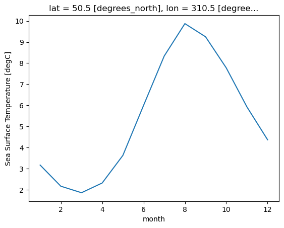
In this example, we plot the zonal mean climatology:

tos_clim.mean(dim='lon').transpose().plot.contourf(levels=12, cmap='turbo');
../../_images/744a94cd827ce2feeb760ab94530647cc9beff3ee90db9bc3a8902c55d59c178.png

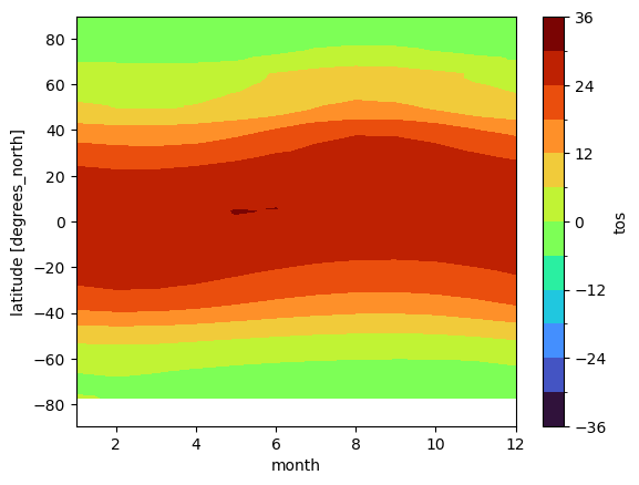
Finally, this example calculates and plots the difference between the climatology for January and the climatology for December:

(tos_clim.sel(month=1) - tos_clim.sel(month=12)).plot(size=6, robust=True);
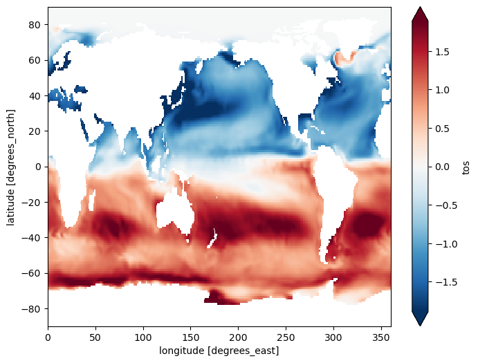
../../_images/54c9c2e758d9c9914b4aca68aa5af780cefb566dcbcb5d2f3884af2c6821447d.png

Compute anomaly

In this example, we compute the anomaly of the original data by removing the climatology from the data values. As shown in previous examples, the climatology is first calculated. The calculated climatology is then removed from the data using arithmetic and Xarray’s groupby method:

gb = ds.tos.groupby('time.month')
tos_anom = gb - gb.mean(dim='time')
tos_anom
<xarray.DataArray 'tos' (time: 180, lat: 180, lon: 360)> Size: 47MB
array([[[        nan,         nan,         nan, ...,         nan,
                 nan,         nan],
        [        nan,         nan,         nan, ...,         nan,
                 nan,         nan],
        [        nan,         nan,         nan, ...,         nan,
                 nan,         nan],
        ...,
        [-0.01402271, -0.01401687, -0.01401365, ..., -0.01406252,
         -0.01404917, -0.01403356],
        [-0.01544118, -0.01544476, -0.01545036, ..., -0.0154475 ,
         -0.01544321, -0.01544082],
        [-0.01638114, -0.01639009, -0.01639998, ..., -0.01635301,
         -0.01636147, -0.01637137]],

       [[        nan,         nan,         nan, ...,         nan,
                 nan,         nan],
        [        nan,         nan,         nan, ...,         nan,
                 nan,         nan],
        [        nan,         nan,         nan, ...,         nan,
                 nan,         nan],
...
        [ 0.01727939,  0.01713431,  0.01698041, ...,  0.0176847 ,
          0.01755834,  0.01742125],
        [ 0.0173862 ,  0.0172919 ,  0.01719594, ...,  0.01766813,
          0.01757395,  0.01748013],
        [ 0.01693714,  0.01687253,  0.01680517, ...,  0.01709175,
          0.0170424 ,  0.01699162]],

       [[        nan,         nan,         nan, ...,         nan,
                 nan,         nan],
        [        nan,         nan,         nan, ...,         nan,
                 nan,         nan],
        [        nan,         nan,         nan, ...,         nan,
                 nan,         nan],
        ...,
        [ 0.01506364,  0.01491845,  0.01476014, ...,  0.01545238,
          0.0153321 ,  0.01520228],
        [ 0.0142287 ,  0.01412642,  0.01402068, ...,  0.0145216 ,
          0.01442552,  0.01432824],
        [ 0.01320827,  0.01314461,  0.01307774, ...,  0.0133611 ,
          0.0133127 ,  0.01326215]]], dtype=float32)
Coordinates:
  * time     (time) object 1kB 2000-01-15 12:00:00 ... 2014-12-15 12:00:00
  * lat      (lat) float64 1kB -89.5 -88.5 -87.5 -86.5 ... 86.5 87.5 88.5 89.5
  * lon      (lon) float64 3kB 0.5 1.5 2.5 3.5 4.5 ... 356.5 357.5 358.5 359.5
    month    (time) int64 1kB 1 2 3 4 5 6 7 8 9 10 11 ... 3 4 5 6 7 8 9 10 11 12
tos_anom.sel(lon=310, lat=50, method='nearest').plot();
../../_images/1ef40d335857fa8fc92493dab3a12ea9523aac3b4715787e87137171cb91ef73.png

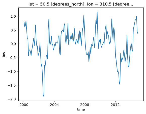
In this example, we compute and plot our dataset’s mean global anomaly over time. In order to specify global data, we must provide both lat and lon to the mean() method’s dim keyword argument:

unweighted_mean_global_anom = tos_anom.mean(dim=['lat', 'lon'])
unweighted_mean_global_anom.plot();
../../_images/296cbdce5356e063165c603b3530a6c74983f2041817c66b2d110a4483a00d7c.png

Many geoscientific algorithms perform operations over data contained in many different grid cells. However, if the grid cells are not equivalent in size, the operation is not scientifically valid by default. Fortunately, this can be fixed by weighting the data in each grid cell by the size of the cell. Weighting data in Xarray is simple, as Xarray has a built-in weighting method, known as .weighted().

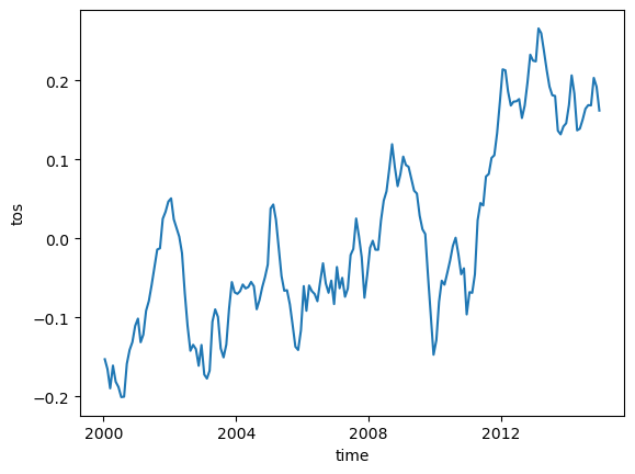
In this example, we again make use of the Pythia example data library to load a new CESM2 dataset. Contained in this dataset are weights corresponding to the grid cells in our anomaly data:

filepath2 = DATASETS.fetch('CESM2_grid_variables.nc')
areacello = xr.open_dataset(filepath2).areacello
areacello
Downloading file 'CESM2_grid_variables.nc' from 'https://github.com/ProjectPythia/pythia-datasets/raw/main/data/CESM2_grid_variables.nc' to '/home/runner/.cache/pythia-datasets'.
<xarray.DataArray 'areacello' (lat: 180, lon: 360)> Size: 518kB
[64800 values with dtype=float64]
Coordinates:
  * lat      (lat) float64 1kB -89.5 -88.5 -87.5 -86.5 ... 86.5 87.5 88.5 89.5
  * lon      (lon) float64 3kB 0.5 1.5 2.5 3.5 4.5 ... 356.5 357.5 358.5 359.5
Attributes: (12/17)
    cell_methods:   area: sum
    comment:        TAREA
    description:    Cell areas for any grid used to report ocean variables an...
    frequency:      fx
    id:             areacello
    long_name:      Grid-Cell Area for Ocean Variables
    ...             ...
    time_label:     None
    time_title:     No temporal dimensions ... fixed field
    title:          Grid-Cell Area for Ocean Variables
    type:           real
    units:          m2
    variable_id:    areacello

In a similar fashion to a previous example, this example calculates mean global anomaly. However, this example makes use of the .weighted() method and the newly loaded CESM2 dataset to weight the grid cell data as described above:

weighted_mean_global_anom = tos_anom.weighted(areacello).mean(dim=['lat', 'lon'])

This example plots both unweighted and weighted mean data, which illustrates the degree of scientific error with unweighted data:

unweighted_mean_global_anom.plot(size=7)
weighted_mean_global_anom.plot()
plt.legend(['unweighted', 'weighted']);
../../_images/e9e07fc7d52a0afdbb4c1769987bdeca7caf514fc915387ff86dd3b58c248a74.png

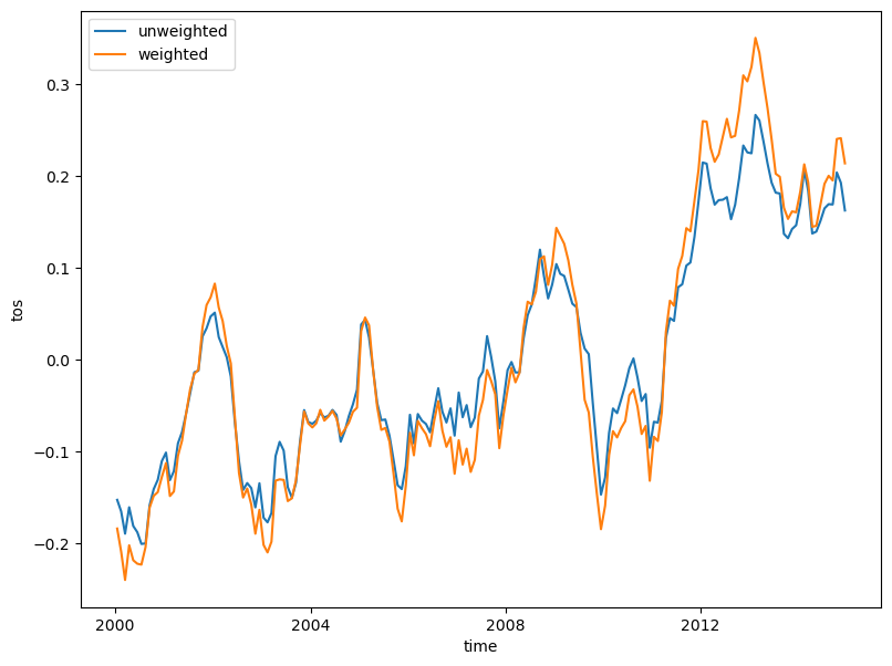
Other high level computation functionality

This example illustrates the resampling of a dataset’s time dimension to annual frequency:

r = ds.tos.resample(time='AS')
r
<string>:6: FutureWarning: 'AS' is deprecated and will be removed in a future version. Please use 'YS' instead of 'AS'.
DataArrayResample, grouped over '__resample_dim__'
15 groups with labels 2000-01-01, 00:00:00, ..., 201....
r.mean()
<xarray.DataArray 'tos' (time: 15, lat: 180, lon: 360)> Size: 4MB
array([[[       nan,        nan,        nan, ...,        nan,
                nan,        nan],
        [       nan,        nan,        nan, ...,        nan,
                nan,        nan],
        [       nan,        nan,        nan, ...,        nan,
                nan,        nan],
        ...,
        [-1.7474419, -1.7474264, -1.7474008, ..., -1.7474308,
         -1.7474365, -1.7474445],
        [-1.7424874, -1.7424612, -1.7424251, ..., -1.742536 ,
         -1.7425283, -1.7425116],
        [-1.7382039, -1.7381679, -1.7381277, ..., -1.7383199,
         -1.7382846, -1.7382454]],

       [[       nan,        nan,        nan, ...,        nan,
                nan,        nan],
        [       nan,        nan,        nan, ...,        nan,
                nan,        nan],
        [       nan,        nan,        nan, ...,        nan,
                nan,        nan],
...
        [-1.6902231, -1.6899008, -1.6895409, ..., -1.6910189,
         -1.6907759, -1.6905178],
        [-1.6879102, -1.6876906, -1.6874666, ..., -1.6885366,
         -1.6883289, -1.688121 ],
        [-1.6883243, -1.6881752, -1.6880217, ..., -1.6886654,
         -1.6885542, -1.6884427]],

       [[       nan,        nan,        nan, ...,        nan,
                nan,        nan],
        [       nan,        nan,        nan, ...,        nan,
                nan,        nan],
        [       nan,        nan,        nan, ...,        nan,
                nan,        nan],
        ...,
        [-1.6893266, -1.6893964, -1.6894479, ..., -1.6889572,
         -1.6890831, -1.6892204],
        [-1.6776317, -1.6777302, -1.6778082, ..., -1.6771463,
         -1.6773272, -1.677492 ],
        [-1.672563 , -1.6726688, -1.6727766, ..., -1.6723493,
         -1.6724195, -1.6724887]]], dtype=float32)
Coordinates:
  * lat      (lat) float64 1kB -89.5 -88.5 -87.5 -86.5 ... 86.5 87.5 88.5 89.5
  * lon      (lon) float64 3kB 0.5 1.5 2.5 3.5 4.5 ... 356.5 357.5 358.5 359.5
  * time     (time) object 120B 2000-01-01 00:00:00 ... 2014-01-01 00:00:00
Attributes: (12/19)
    cell_measures:  area: areacello
    cell_methods:   area: mean where sea time: mean
    comment:        Model data on the 1x1 grid includes values in all cells f...
    description:    This may differ from "surface temperature" in regions of ...
    frequency:      mon
    id:             tos
    ...             ...
    time_label:     time-mean
    time_title:     Temporal mean
    title:          Sea Surface Temperature
    type:           real
    units:          degC
    variable_id:    tos

This example illustrates using the rolling method to compute averages in a moving window of 5 months of data:

m_avg = ds.tos.rolling(time=5, center=True).mean()
m_avg
<xarray.DataArray 'tos' (time: 180, lat: 180, lon: 360)> Size: 47MB
array([[[       nan,        nan,        nan, ...,        nan,
                nan,        nan],
        [       nan,        nan,        nan, ...,        nan,
                nan,        nan],
        [       nan,        nan,        nan, ...,        nan,
                nan,        nan],
        ...,
        [       nan,        nan,        nan, ...,        nan,
                nan,        nan],
        [       nan,        nan,        nan, ...,        nan,
                nan,        nan],
        [       nan,        nan,        nan, ...,        nan,
                nan,        nan]],

       [[       nan,        nan,        nan, ...,        nan,
                nan,        nan],
        [       nan,        nan,        nan, ...,        nan,
                nan,        nan],
        [       nan,        nan,        nan, ...,        nan,
                nan,        nan],
...
        [       nan,        nan,        nan, ...,        nan,
                nan,        nan],
        [       nan,        nan,        nan, ...,        nan,
                nan,        nan],
        [       nan,        nan,        nan, ...,        nan,
                nan,        nan]],

       [[       nan,        nan,        nan, ...,        nan,
                nan,        nan],
        [       nan,        nan,        nan, ...,        nan,
                nan,        nan],
        [       nan,        nan,        nan, ...,        nan,
                nan,        nan],
        ...,
        [       nan,        nan,        nan, ...,        nan,
                nan,        nan],
        [       nan,        nan,        nan, ...,        nan,
                nan,        nan],
        [       nan,        nan,        nan, ...,        nan,
                nan,        nan]]], dtype=float32)
Coordinates:
  * time     (time) object 1kB 2000-01-15 12:00:00 ... 2014-12-15 12:00:00
  * lat      (lat) float64 1kB -89.5 -88.5 -87.5 -86.5 ... 86.5 87.5 88.5 89.5
  * lon      (lon) float64 3kB 0.5 1.5 2.5 3.5 4.5 ... 356.5 357.5 358.5 359.5
Attributes: (12/19)
    cell_measures:  area: areacello
    cell_methods:   area: mean where sea time: mean
    comment:        Model data on the 1x1 grid includes values in all cells f...
    description:    This may differ from "surface temperature" in regions of ...
    frequency:      mon
    id:             tos
    ...             ...
    time_label:     time-mean
    time_title:     Temporal mean
    title:          Sea Surface Temperature
    type:           real
    units:          degC
    variable_id:    tos
lat = 50
lon = 310

m_avg.isel(lat=lat, lon=lon).plot(size=6)
ds.tos.isel(lat=lat, lon=lon).plot()
plt.legend(['5-month moving average', 'monthly data']);
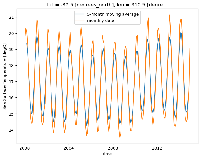
../../_images/6e570983369c5e29eb77847abfb5743a612e8e39cea91602438cd3d031964765.png

Masking Data

Masking of data can be performed in Xarray by providing single or multiple conditions to either Xarray’s .where() method or a Dataset or DataArray’s .where() method. Data values matching the condition(s) are converted into a single example value, effectively masking them from the scientifically important data. In the following set of examples, we use the .where() method to mask various data values in the tos DataArray.

For reference, we will first print our entire sea-surface temperature (SST) dataset:

ds
<xarray.Dataset> Size: 47MB
Dimensions:    (time: 180, d2: 2, lat: 180, lon: 360)
Coordinates:
  * time       (time) object 1kB 2000-01-15 12:00:00 ... 2014-12-15 12:00:00
  * lat        (lat) float64 1kB -89.5 -88.5 -87.5 -86.5 ... 86.5 87.5 88.5 89.5
  * lon        (lon) float64 3kB 0.5 1.5 2.5 3.5 4.5 ... 356.5 357.5 358.5 359.5
Dimensions without coordinates: d2
Data variables:
    time_bnds  (time, d2) object 3kB ...
    lat_bnds   (lat, d2) float64 3kB ...
    lon_bnds   (lon, d2) float64 6kB ...
    tos        (time, lat, lon) float32 47MB nan nan nan ... -1.746 -1.746
Attributes: (12/45)
    Conventions:            CF-1.7 CMIP-6.2
    activity_id:            CMIP
    branch_method:          standard
    branch_time_in_child:   674885.0
    branch_time_in_parent:  219000.0
    case_id:                972
    ...                     ...
    sub_experiment_id:      none
    table_id:               Omon
    tracking_id:            hdl:21.14100/2975ffd3-1d7b-47e3-961a-33f212ea4eb2
    variable_id:            tos
    variant_info:           CMIP6 20th century experiments (1850-2014) with C...
    variant_label:          r11i1p1f1

Using where with one condition

In this set of examples, we are trying to analyze data at the last temporal value in the dataset. This first example illustrates the use of .isel() to perform this analysis:

sample = ds.tos.isel(time=-1)
sample
<xarray.DataArray 'tos' (lat: 180, lon: 360)> Size: 259kB
array([[      nan,       nan,       nan, ...,       nan,       nan,       nan],
       [      nan,       nan,       nan, ...,       nan,       nan,       nan],
       [      nan,       nan,       nan, ...,       nan,       nan,       nan],
       ...,
       [-1.756119, -1.756165, -1.756205, ..., -1.755922, -1.755986, -1.756058],
       [-1.750638, -1.750658, -1.750667, ..., -1.750508, -1.750561, -1.750605],
       [-1.74627 , -1.746267, -1.746261, ..., -1.746309, -1.746299, -1.746285]],
      dtype=float32)
Coordinates:
    time     object 8B 2014-12-15 12:00:00
  * lat      (lat) float64 1kB -89.5 -88.5 -87.5 -86.5 ... 86.5 87.5 88.5 89.5
  * lon      (lon) float64 3kB 0.5 1.5 2.5 3.5 4.5 ... 356.5 357.5 358.5 359.5
Attributes: (12/19)
    cell_measures:  area: areacello
    cell_methods:   area: mean where sea time: mean
    comment:        Model data on the 1x1 grid includes values in all cells f...
    description:    This may differ from "surface temperature" in regions of ...
    frequency:      mon
    id:             tos
    ...             ...
    time_label:     time-mean
    time_title:     Temporal mean
    title:          Sea Surface Temperature
    type:           real
    units:          degC
    variable_id:    tos

As shown in the previous example, methods like .isel() and .sel() return data of a different shape than the original data provided to them. However, .where() preserves the shape of the original data by masking the values with a Boolean condition. Data values for which the condition is True are returned identical to the values passed in. On the other hand, data values for which the condition is False are returned as a preset example value. (This example value defaults to nan, but can be set to other values as well.)

Before testing .where(), it is helpful to look at the official documentation. As stated above, the .where() method takes a Boolean condition. (Boolean conditions use operators such as less-than, greater-than, and equal-to, and return a value of True or False.) Most uses of .where() check whether or not specific data values are less than or greater than a constant value. As stated in the documentation, the data values specified in the Boolean condition of .where() can be any of the following:

  • a DataArray

  • a Dataset

  • a function

In the following example, we make use of .where() to mask data with temperature values greater than 0. Therefore, values greater than 0 are set to nan, as described above. (It is important to note that the Boolean condition matches values to keep, not values to mask out.)

masked_sample = sample.where(sample < 0.0)
masked_sample
<xarray.DataArray 'tos' (lat: 180, lon: 360)> Size: 259kB
array([[       nan,        nan,        nan, ...,        nan,        nan,
               nan],
       [       nan,        nan,        nan, ...,        nan,        nan,
               nan],
       [       nan,        nan,        nan, ...,        nan,        nan,
               nan],
       ...,
       [-1.7561191, -1.7561648, -1.7562052, ..., -1.7559224, -1.7559862,
        -1.7560585],
       [-1.7506379, -1.7506577, -1.7506672, ..., -1.7505083, -1.750561 ,
        -1.7506049],
       [-1.7462697, -1.7462667, -1.7462606, ..., -1.7463093, -1.746299 ,
        -1.7462848]], dtype=float32)
Coordinates:
    time     object 8B 2014-12-15 12:00:00
  * lat      (lat) float64 1kB -89.5 -88.5 -87.5 -86.5 ... 86.5 87.5 88.5 89.5
  * lon      (lon) float64 3kB 0.5 1.5 2.5 3.5 4.5 ... 356.5 357.5 358.5 359.5
Attributes: (12/19)
    cell_measures:  area: areacello
    cell_methods:   area: mean where sea time: mean
    comment:        Model data on the 1x1 grid includes values in all cells f...
    description:    This may differ from "surface temperature" in regions of ...
    frequency:      mon
    id:             tos
    ...             ...
    time_label:     time-mean
    time_title:     Temporal mean
    title:          Sea Surface Temperature
    type:           real
    units:          degC
    variable_id:    tos

In this example, we use Matplotlib to plot the original, unmasked data, as well as the masked data created in the previous example.

fig, axes = plt.subplots(ncols=2, figsize=(19, 6))
sample.plot(ax=axes[0])
masked_sample.plot(ax=axes[1]);
../../_images/e80681079b231135b15ac59f11233357b279b29c002d04e31b20fe5d3f75b0e0.png

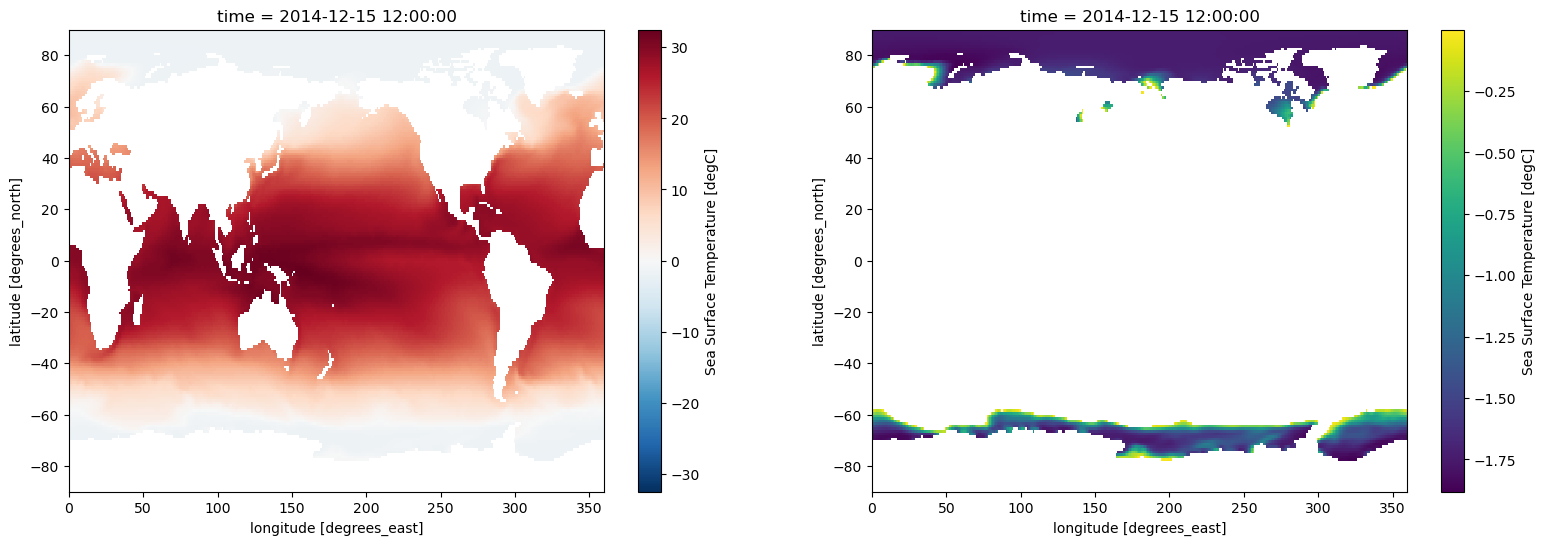
Using where with multiple conditions

Those familiar with Boolean conditions know that such conditions can be combined by using logical operators. In the case of .where(), the relevant logical operators are bitwise or exclusive 'and' (represented by the & symbol) and bitwise or exclusive ‘or’ (represented by the | symbol). This allows multiple masking conditions to be specified in a single use of .where(); however, be aware that if multiple conditions are specified in this way, each simple Boolean condition must be enclosed in parentheses. (If you are not familiar with Boolean conditions, or this section is confusing in any way, please review a detailed Boolean expression guide before continuing with the tutorial.) In this example, we provide multiple conditions to .where() using a more complex Boolean condition. This allows us to mask locations with temperature values less than 25, as well as locations with temperature values greater than 30. (As stated above, the Boolean condition matches values to keep, and everything else is masked out. Because we are now using more complex Boolean conditions, understanding the following example may be difficult. Please review a Boolean condition guide if needed.)

sample.where((sample > 25) & (sample < 30)).plot(size=6);
../../_images/a95c64364491de03c669d4e365813e39c907d610292e31c1c911d8278caf3a68.png

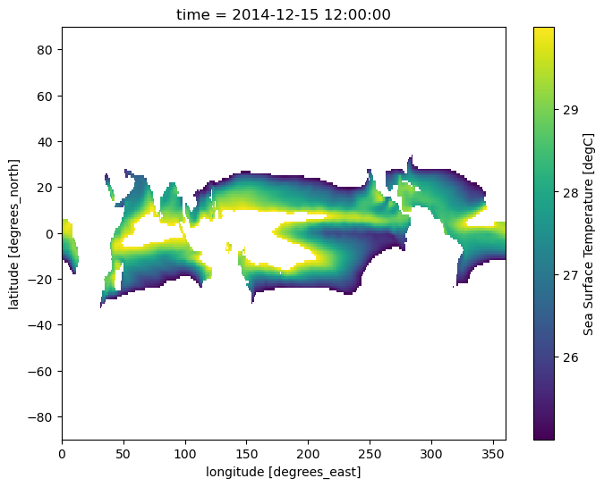
In addition to using DataArrays and Datasets in Boolean conditions provided to .where(), we can also use coordinate variables. In the following example, we make use of Boolean conditions containing latitude and longitude coordinates. This greatly simplifies the masking of regions outside of the Niño 3.4 region:

sample.where(
    (sample.lat < 5) & (sample.lat > -5) & (sample.lon > 190) & (sample.lon < 240)
).plot(size=6);
../../_images/bc1de77ab4b6647d3490d41f003e9efea5a7dce7cc12f152c9b1f1e615daf36c.png

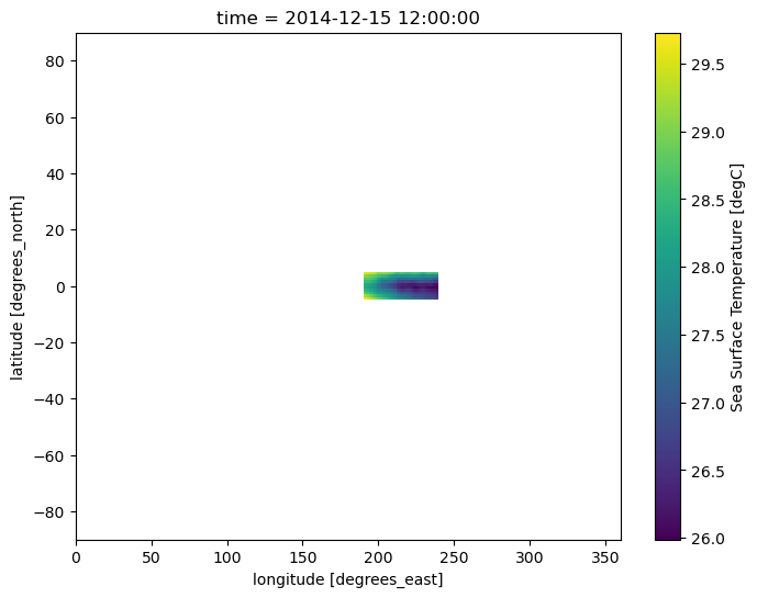
Using where with a custom fill value

In the previous examples that make use of .where(), the masked data values are set to nan. However, this behavior can be modified by providing a second value, in numeric form, to .where(); if this numeric value is provided, it will be used instead of nan for masked data values. In this example, masked data values are set to 0 by providing a second value of 0 to the .where() method:

sample.where((sample > 25) & (sample < 30), 0).plot(size=6);
../../_images/3cf69c70f2646c79a40649eb5bb76a0ce4260a1fdc632a2828beceed66cdcc1b.png

Summary

  • In a similar manner to NumPy arrays, performing arithmetic on a DataArray affects all values simultaneously.

  • Xarray allows for simple data aggregation, over single or multiple dimensions, by way of built-in methods such as sum() and mean().

  • Xarray supports the useful split-apply-combine workflow through the groupby method.

  • Xarray allows replacing (masking) of data matching specific Boolean conditions by means of the .where() method.

What’s next?

The next tutorial illustrates the use of previously covered Xarray concepts in a geoscientifically relevant example: plotting the Niño 3.4 Index.

Resources and References