Overview
Jupyter Notebooks (*.ipynb files) are computational narrative documents that can contain executable code, LaTeX equations, visualizations (e.g., plots, pictures), and richly formatted text. Jupyter Notebooks are celebrated for their interactive output that allows movement between code, code output, explanations, and more code — similar to how scientists think and solve problems. Jupyter Notebooks can be thought of as a living, runnable publication and make for a great presentation platform.
This section introduces the notebook interface within JupyterLab, and basic features of notebook creation, editing, and execution.
Prerequisites
| Concepts | Importance | Notes |
|---|---|---|
| Getting Started with Jupyter | Helpful | |
| Installing and Running Python: Python in Jupyter | Helpful | |
| A JupyterLab Tour | Helpful |
The notebook interface
There are two ways to open a Jupyter Notebook. One way is to select the File Browser Tab, click the “New Launcher” button, and select a Python 3 Notebook from the Launcher. Another way is to go to the top Menu Bar and select “File ▶ New ▶ Notebook”. JupyterLab will prompt you with a dialogue box to select the Kernel you want to use in your Notebook. Select the “Python 3” kernel.
If you have the File Browser Tab open, notice you just created a file called Untitled.ipynb. You will also have a new window open in the main work area for your new Notebook.
Let’s explore the Notebook interface:
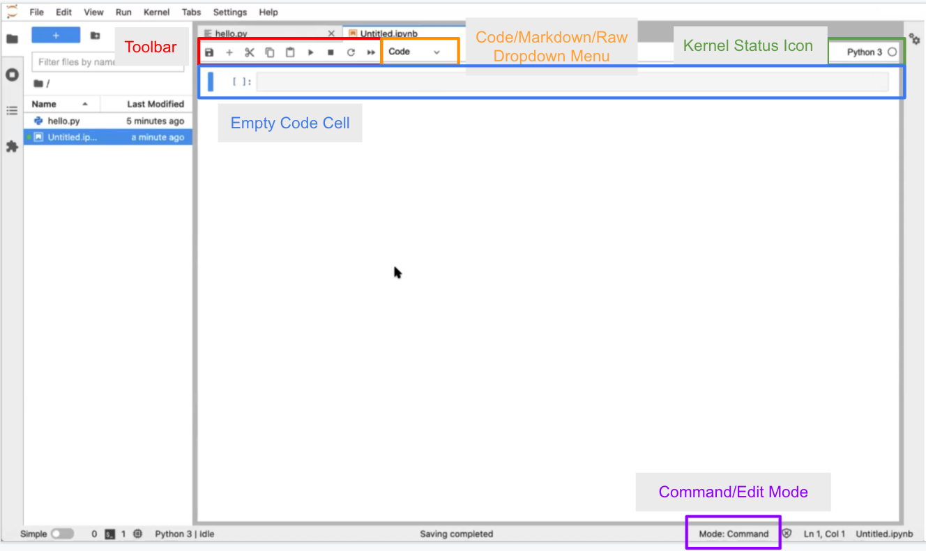
There is a Toolbar at the top with buttons that allow you to Save, Create New Cells, Cut/Paste/Copy Cells, Run the Cell, Stop the Kernel, and Refresh the Kernel. There is also a dropdown menu to select the kind of cell (Markdown, Raw, or Code). All the way to the right is the name of your Kernel (which you can click to change Kernels) and a Kernel Status Icon that indicates if something is being computed by the Kernel (by a dark circle) or not (by an empty circle).
Below the Toolbar is the Notebook itself. You should see an empty cell at the top of the Notebook. This should look similar to the layout of the Console.
The cell can be in 1 of 2 modes: command mode or edit mode. If your cell is grayed out and you can’t see a blinking cursor in the cell, then the cell is in command mode. We’ll talk about command mode more later. Click inside the box, and the cell will turn white with a blinking cursor inside it; the cell is now in edit mode. The mode is also listed on the info bar at the bottom of the page. The cell is selected if the blue bar is on the left side of the cell.
You may move the Notebook over so you can see your text file at the same time to compare, resizing the Notebook window as needed.
Code cells
New cells default to the Code type. Each Code cell is a free-standing Python script that can be executed directly in the notebook. Here are some “getting started” steps:
Create simple Python scripts in code cells
Click inside the first cell of the Notebook to switch the cell to edit mode. Enter the following into the cell:
print(2+2)Then type Shift+Enter to execute the cell.
You’ll see the output, 4, printed directly below your code cell. Executing the cell automatically creates a new cell in edit mode below the first.
In this new cell, enter:
for i in range(4):
    print(i)
Execute the cell. A Jupyter code cell can run multiple lines of code; each Jupyter code cell can even contain a complete Python program!
Using import statements in code cells
Just like any other Python execution environment, the import statement will bring the contents of other Python modules into the current workspace.
Assuming you created a file hello.py in the previous lesson A JupyterLab Tour, you can now import this code into your notebook. Enter the following into the next cell:
import helloThen type Shift+Enter.
This single-line import statement runs the contents of your hello.py script file, and would do the same for any file regardless of length.
You’ve executed the cell with the Python 3 kernel, and it spit out the output, Hello, World!.
Since you’ve imported the hello.py module into the Notebook’s kernel runtime, you can now directly look at the variable s in this second cell.
Enter the following in the next cell:
hello.sHit Shift+Enter to execute.
Again, it displays the value of the variable s from the “hello” module we just created. One difference is that this time the output is given its own label [2] matching the input label of the cell (whereas the output from cell [1] is not labelled). This is the difference between output sent to the screen vs. the return value of the cell.
Importing standard library modules
Let’s now import a module from the Python standard library:
import time
time.sleep(10)
Again, hit Shift+Enter.
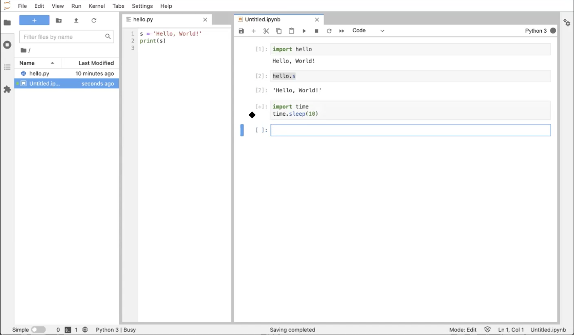
The time.sleep(10) function causes code to wait for 10 seconds, which is plenty of time to notice how the cell changes in time:
The label of the cell is
[*], indicating that the kernel is running that cellIn the top right corner of the Notebook, the status icon is a filled-in circle, indicating that the kernel is running
After 10 seconds, the cell completes running, the label is updated to [3], and the status icon returns to the “empty circle” state. If you rerun the cell, the label will update to [4].
Markdown cells
Markdown cells are used for formatted rich text. Markdown is a markup language that allows you to format text in a plain-text editor, which is then rendered as visually rich web output.
Here we will demonstrate some common Markdown syntax. You can learn more at the Markdown Guide site or in our Getting Started with Jupyter: Markdown content.
Create a Markdown cell
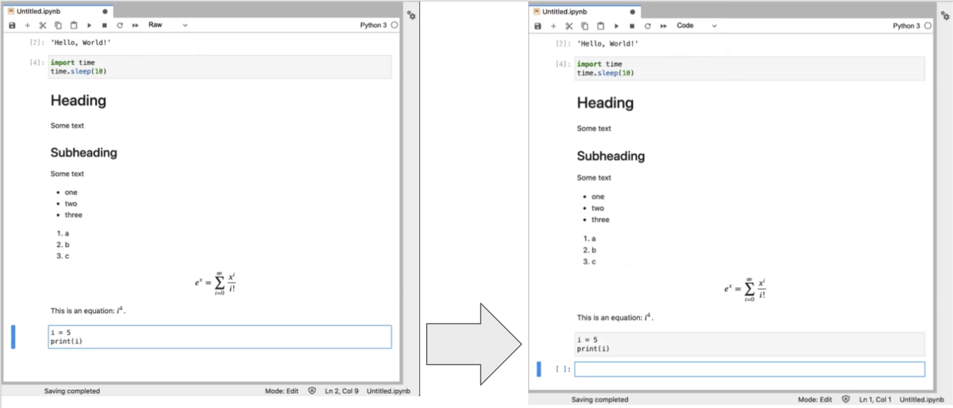
Now, with the next cell selected (i.e., the blue bar appears to the left of the cell), whether in edit or command mode, go up to the “cell type” dropdown menu above and select “Markdown”.
Notice that the [ ] label goes away.
Hierarchical section headings and lists
Click on the cell and enter edit mode; we can now type in some markdown text like so:
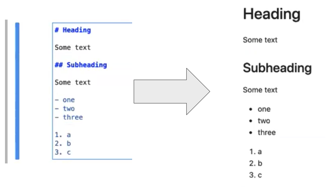
# This is a heading!
And this is some text.

## And this is a subheading
with a bulleted list in it:

 - one
 - two
 - three
Then press Shift+Enter to render the markdown to HTML.
Math in a Markdown cell
Again, in the next cell, change the cell type to “Markdown”. To demonstrate displaying equations, enter:
## Some math
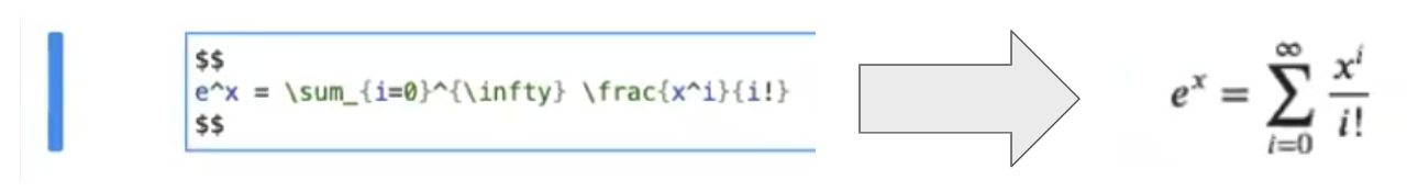
And Jupyter’s version of markdown can display LaTeX:
$$
e^x=\sum_{i=0}^{\infty} \frac{1}{i!}x^i
$$When you are done, type Shift+Enter to render the markdown document.
You can also do inline equations with a single “$”, for example
This is an equation: $i^4$.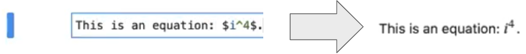
Note that the “Markdown” source code is rendered into much prettier text, which we can take advantage of for narrating our work in the Notebook!
Raw cells
Now in a new cell selected, select “raw” from the “cell type” dropdown menu. Again, the [ ] label goes away, and you can enter the following in the cell:
i = 8
print(i)
When you Shift+Enter the text isn’t rendered.
This is a way of entering text/source that you do not want the Notebook to do anything with (i.e., no rendering).
Beyond the basics
Here are a handful of other things you can do with notebook cells in JupyterLab.
Command mode shortcuts
Try selecting the “raw” cell you just created by clicking on the far left of the cell.
You are now in “command mode”. The up and down arrows move to different cells. Don’t hit Enter which would switch the cell to “edit mode." Let’s explore command mode.
You can change the cell type with y for code, m for markdown, or r for raw.
You can add a new cell above the selected cell with a (or below the selected cell with b).
You can cut (x), copy (c), and paste (v).
You can move a cell up or down by clicking and dragging.
Special variables
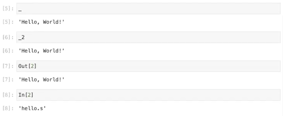
Now, in the empty cell at the end, enter one underscore:
_This is a special character that means the last cell output. Two underscores means the second to last cell output, and three underscores means the third to last output. You can also refer to the output by label with:
_2You can equivalently use the variables Out[2] or In[2] to retrieve the output and input (as a string).
Shell commands
In the next code cell, enter the following:
!pwdThe ! allows you to write shell commands. A shell command is a command that is run by the host operating system, not the Python kernel. Executing this cell will “print the working directory” (i.e. your current directory).
You can even use the output of shell commands as input to Python code. For example:
files = !ls
print(files)
Stopping & restarting the kernel
All of your commands and their output have been remembered by the kernel. However, sometimes you may get code that takes too long to execute, and you need to stop it. For example, in the next code cell, run:
time.sleep(1000)You can stop the kernel with the square “stop” button at the top Notebook toolbar. This results in a KeyboardInterrupt error.
If you execute a notebook out of order, you can end up in a corrupted state (redefined variables, for example). To start fresh, you should restart the kernel with the circle-arrow button in the toolbar at the top. Now the kernel has forgotten everything, and you’ll need to rerun each cell.
Magics
A “magic” is a Jupyter Notebook command proceded by a % symbol. In the next code cell, enter the following:
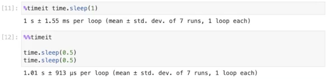
%timeit time.sleep(1)The %timeit magic is a timer that runs the command multiple times, measuring how long it takes and gathering timing statistics. Hit Shift+Enter to see it work.
Multiline magics work on entire cells, and these have a double-%. For example, here is a multiline version of the timeit magic:
%%timeit

time.sleep(0.5)
time.sleep(0.5)
Then press Shift+Enter to run it. This will time the entire cell.
Shutting down
Before shutting down, save your notebook with the disc icon in the Notebook toolbar. Now, close both tabs (the notebook and the text editor). You’re back to the Launcher.
The notebook kernel is still running, though, so go to the Running Kernels tab and shut it down.
Now we’re done. Go to “File ▶ Shut Down” to close both your browser tab and JupyterLab itself.
Summary
You are now familiar with creating and running Jupyter Notebooks in the JupyterLab interface. Jupyter is popular for allowing you to create rich computational narratives by interspersing Markdown text or equations between code cells. JupyterLab also offers some functionality that a Python script does not: certain keyboard shortcuts, special variables, shell scripting, and magics.