Intermediate NumPy
Overview
Working with multiple dimensions
Subsetting of irregular arrays with booleans
Sorting, or indexing with indices
Prerequisites
Concepts |
Importance |
Notes |
|---|---|---|
Necessary |
Time to learn: 20 minutes
Imports
We will be including Matplotlib to illustrate some of our examples, but you don’t need knowledge of it to complete this notebook.
import matplotlib.pyplot as plt
import numpy as np
Using axes to slice arrays
Here we introduce an important concept when working with NumPy: the axis. This indicates the particular dimension along which a function should operate (provided the function does something taking multiple values and converts to a single value).
Let’s look at a concrete example with sum:
a = np.arange(12).reshape(3, 4)
a
array([[ 0,  1,  2,  3],
       [ 4,  5,  6,  7],
       [ 8,  9, 10, 11]])
This calculates the total of all values in the array.
np.sum(a)
np.int64(66)
Info
Some of NumPy’s functions can be accessed as ndarray methods!
a.sum()
np.int64(66)
Now, with a reminder about how our array is shaped,
a.shape
(3, 4)
we can specify axis to get just the sum across each of our rows.
np.sum(a, axis=0)
array([12, 15, 18, 21])
Or do the same and take the sum across columns:
np.sum(a, axis=1)
array([ 6, 22, 38])
After putting together some data and introducing some more advanced calculations, let’s demonstrate a multi-layered example: calculating temperature advection. If you’re not familiar with this (don’t worry!), we’ll be looking to calculate
and to do so we’ll start with some random \(T\) and \(\vec{v}\) values,
temp = np.random.randn(100, 50)
u = np.random.randn(100, 50)
v = np.random.randn(100, 50)
We can calculate the np.gradient of our new \(T(100x50)\) field as two separate component gradients,
gradient_x, gradient_y = np.gradient(temp)
In order to calculate \(-\vec{v} \cdot \nabla T\), we will use np.dstack to turn our two separate component gradient fields into one multidimensional field containing \(x\) and \(y\) gradients at each of our \(100x50\) points,
grad_vectors = np.dstack([gradient_x, gradient_y])
print(grad_vectors.shape)
(100, 50, 2)
and then do the same for our separate \(u\) and \(v\) wind components,
wind_vectors = np.dstack([u, v])
print(wind_vectors.shape)
(100, 50, 2)
Finally, we can calculate the dot product of these two multidimensional fields of wind and temperature gradient components by hand as an element-wise multiplication, *, and then a sum of our separate components at each point (i.e., along the last axis),
advection = (wind_vectors * -grad_vectors).sum(axis=-1)
print(advection.shape)
(100, 50)
Indexing arrays with boolean values
Array comparisons
NumPy can easily create arrays of boolean values and use those to select certain values to extract from an array
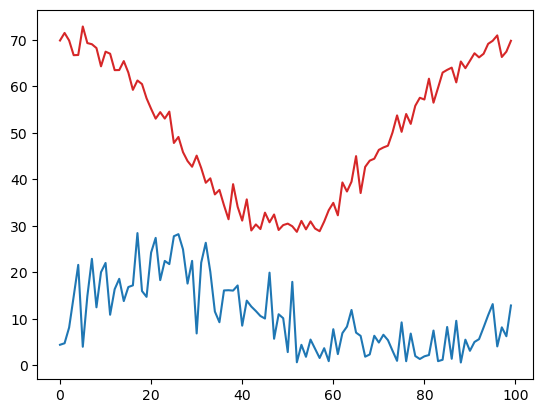
# Create some synthetic data representing temperature and wind speed data
np.random.seed(19990503)  # Make sure we all have the same data
temp = 20 * np.cos(np.linspace(0, 2 * np.pi, 100)) + 50 + 2 * np.random.randn(100)
speed = np.abs(
    10 * np.sin(np.linspace(0, 2 * np.pi, 100)) + 10 + 5 * np.random.randn(100)
)
plt.plot(temp, 'tab:red')
plt.plot(speed, 'tab:blue');

By doing a comparison between a NumPy array and a value, we get an array of values representing the results of the comparison between each element and the value
temp > 45
array([ True,  True,  True,  True,  True,  True,  True,  True,  True,
        True,  True,  True,  True,  True,  True,  True,  True,  True,
        True,  True,  True,  True,  True,  True,  True,  True,  True,
        True, False, False,  True, False, False, False, False, False,
       False, False, False, False, False, False, False, False, False,
       False, False, False, False, False, False, False, False, False,
       False, False, False, False, False, False, False, False, False,
       False, False,  True, False, False, False, False,  True,  True,
        True,  True,  True,  True,  True,  True,  True,  True,  True,
        True,  True,  True,  True,  True,  True,  True,  True,  True,
        True,  True,  True,  True,  True,  True,  True,  True,  True,
        True])
This, which is its own NumPy array of boolean values, can be used as an index to another array of the same size. We can even use it as an index within the original temp array we used to compare,
temp[temp > 45]
array([69.89825854, 71.52313905, 69.90028363, 66.73828667, 66.77980233,
       72.91468564, 69.34603239, 69.09533591, 68.27350814, 64.33916721,
       67.49497791, 67.05282372, 63.51829518, 63.54034678, 65.46576463,
       62.99683836, 59.27662304, 61.29361272, 60.51641586, 57.46048995,
       55.19793004, 53.07572989, 54.47998158, 53.09552107, 54.59037269,
       47.84272747, 49.1435589 , 45.87151534, 45.11976794, 45.009292  ,
       46.36021141, 46.87557425, 47.25668992, 50.09599544, 53.77789358,
       50.24073197, 54.07629059, 51.95065202, 55.84827794, 57.56967086,
       57.19572063, 61.67658285, 56.51474577, 59.72166924, 62.99403256,
       63.57569453, 64.05984232, 60.88258643, 65.37759899, 63.94115754,
       65.53070256, 67.15175649, 66.26468701, 67.03811793, 69.17773618,
       69.83571708, 70.99586742, 66.34971928, 67.49905207, 69.83593609])
Info
This only returns the values from our original array meeting the indexing conditions, nothing more! Note the size,
temp[temp > 45].shape
(60,)
Warning
Indexing arrays with arrays requires them to be the same size!
If we store this array somewhere new,
temp_45 = temp[temp > 45]
temp_45[temp < 45]
---------------------------------------------------------------------------
IndexError                                Traceback (most recent call last)
Cell In[19], line 1
----> 1 temp_45[temp < 45]

IndexError: boolean index did not match indexed array along axis 0; size of axis is 60 but size of corresponding boolean axis is 100
We find that our original (100,) shape array is too large to subset our new (60,) array.
If their sizes do match, the boolean array can come from a totally different array!
speed > 10
array([False, False, False,  True,  True, False,  True,  True,  True,
        True,  True,  True,  True,  True,  True,  True,  True,  True,
        True,  True,  True,  True,  True,  True,  True,  True,  True,
        True,  True,  True, False,  True,  True,  True,  True, False,
        True,  True,  True,  True, False,  True,  True,  True,  True,
        True,  True, False,  True,  True, False,  True, False, False,
       False, False, False, False, False, False, False, False, False,
       False,  True, False, False, False, False, False, False, False,
       False, False, False, False, False, False, False, False, False,
       False, False, False, False, False, False, False, False, False,
       False, False, False, False,  True,  True, False, False, False,
        True])
temp[speed > 10]
array([66.73828667, 66.77980233, 69.34603239, 69.09533591, 68.27350814,
       64.33916721, 67.49497791, 67.05282372, 63.51829518, 63.54034678,
       65.46576463, 62.99683836, 59.27662304, 61.29361272, 60.51641586,
       57.46048995, 55.19793004, 53.07572989, 54.47998158, 53.09552107,
       54.59037269, 47.84272747, 49.1435589 , 45.87151534, 43.95971516,
       42.72814762, 42.45316175, 39.2797517 , 40.23351938, 36.77179678,
       34.43329229, 31.42277612, 38.97505745, 34.10549575, 35.70826448,
       29.01276068, 30.31180935, 29.31602671, 32.84580454, 30.76695309,
       29.11344716, 30.16652571, 29.91513049, 39.51784389, 69.17773618,
       69.83571708, 69.83593609])
Replacing values
To extend this, we can use this conditional indexing to assign new values to certain positions within our array, somewhat like a masking operation.
# Make a copy so we don't modify the original data
temp2 = temp.copy()
speed2 = speed.copy()

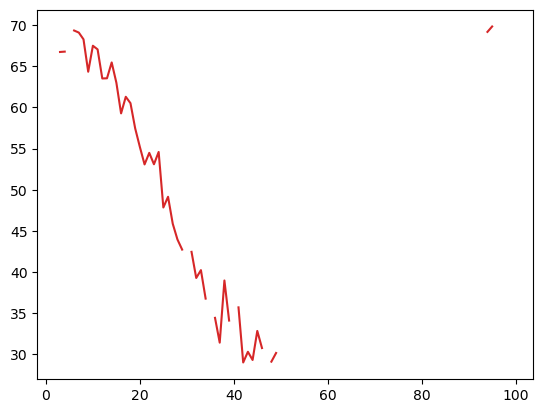
# Replace all places where speed is <10 with NaN (not a number)
temp2[speed < 10] = np.nan
speed2[speed < 10] = np.nan
plt.plot(temp2, 'tab:red');

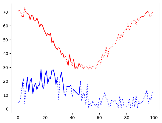
and to put this in context,
plt.plot(temp, 'r:')
plt.plot(temp2, 'r')
plt.plot(speed, 'b:')
plt.plot(speed2, 'b');

If we use parentheses to preserve the order of operations, we can combine these conditions with other bitwise operators like the & for bitwise_and,
multi_mask = (temp < 45) & (speed > 10)
multi_mask
array([False, False, False, False, False, False, False, False, False,
       False, False, False, False, False, False, False, False, False,
       False, False, False, False, False, False, False, False, False,
       False,  True,  True, False,  True,  True,  True,  True, False,
        True,  True,  True,  True, False,  True,  True,  True,  True,
        True,  True, False,  True,  True, False,  True, False, False,
       False, False, False, False, False, False, False, False, False,
       False,  True, False, False, False, False, False, False, False,
       False, False, False, False, False, False, False, False, False,
       False, False, False, False, False, False, False, False, False,
       False, False, False, False, False, False, False, False, False,
       False])
temp[multi_mask]
array([43.95971516, 42.72814762, 42.45316175, 39.2797517 , 40.23351938,
       36.77179678, 34.43329229, 31.42277612, 38.97505745, 34.10549575,
       35.70826448, 29.01276068, 30.31180935, 29.31602671, 32.84580454,
       30.76695309, 29.11344716, 30.16652571, 29.91513049, 39.51784389])
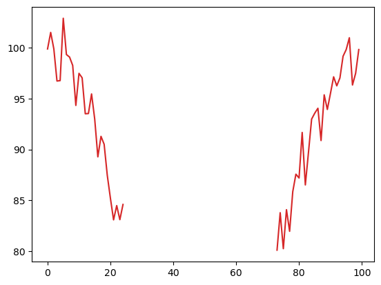
Heat index is only defined for temperatures >= 80F and relative humidity values >= 40%. Using the data generated below, we can use boolean indexing to extract the data where heat index has a valid value.
# Here's the "data"
np.random.seed(19990503)
temp = 20 * np.cos(np.linspace(0, 2 * np.pi, 100)) + 80 + 2 * np.random.randn(100)
relative_humidity = np.abs(
    20 * np.cos(np.linspace(0, 4 * np.pi, 100)) + 50 + 5 * np.random.randn(100)
)

# Create a mask for the two conditions described above
good_heat_index = (temp >= 80) & (relative_humidity >= 0.4)

# Use this mask to grab the temperature and relative humidity values that together
# will give good heat index values
print(temp[good_heat_index])
[ 99.89825854 101.52313905  99.90028363  96.73828667  96.77980233
 102.91468564  99.34603239  99.09533591  98.27350814  94.33916721
  97.49497791  97.05282372  93.51829518  93.54034678  95.46576463
  92.99683836  89.27662304  91.29361272  90.51641586  87.46048995
  85.19793004  83.07572989  84.47998158  83.09552107  84.59037269
  80.09599544  83.77789358  80.24073197  84.07629059  81.95065202
  85.84827794  87.56967086  87.19572063  91.67658285  86.51474577
  89.72166924  92.99403256  93.57569453  94.05984232  90.88258643
  95.37759899  93.94115754  95.53070256  97.15175649  96.26468701
  97.03811793  99.17773618  99.83571708 100.99586742  96.34971928
  97.49905207  99.83593609]
Another bitwise operator we can find helpful is Python’s ~ complement operator, which can give us the inverse of our specific mask to let us assign np.nan to every value not satisfied in good_heat_index.
plot_temp = temp.copy()
plot_temp[~good_heat_index] = np.nan
plt.plot(plot_temp, 'tab:red');

Indexing using arrays of indices
You can also use a list or array of indices to extract particular values–this is a natural extension of the regular indexing. For instance, just as we can select the first element:
temp[0]
np.float64(99.89825854468695)
We can also extract the first, fifth, and tenth elements as a list:
temp[[0, 4, 9]]
array([99.89825854, 96.77980233, 94.33916721])
One of the ways this comes into play is trying to sort NumPy arrays using argsort. This function returns the indices of the array that give the items in sorted order. So for our temp,
inds = np.argsort(temp)
inds
array([52, 57, 42, 48, 54, 44, 56, 51, 49, 43, 50, 46, 58, 55, 53, 40, 37,
       61, 47, 45, 59, 39, 36, 60, 41, 34, 66, 63, 35, 38, 32, 62, 64, 33,
       31, 67, 29, 28, 68, 69, 65, 30, 27, 70, 71, 72, 25, 26, 73, 75, 77,
       21, 23, 74, 76, 22, 24, 20, 78, 82, 80, 19, 79, 16, 83, 18, 87, 17,
       81, 84, 15, 12, 13, 85, 89, 86,  9, 88, 14, 90, 92, 97,  3,  4, 93,
       11, 91, 10, 98,  8,  7, 94,  6, 95, 99,  0,  2, 96,  1,  5])
i.e., our lowest value is at index 52, next 57, and so on. We can use this array of indices as an index for temp,
temp[inds]
array([ 58.71828204,  58.85269149,  59.01276068,  59.11344716,
        59.25186164,  59.31602671,  59.42796381,  59.91513049,
        60.16652571,  60.31180935,  60.48608715,  60.76695309,
        60.93380275,  60.95814392,  61.07199963,  61.1341411 ,
        61.42277612,  62.27369636,  62.44927684,  62.84580454,
        63.37573713,  64.10549575,  64.43329229,  64.95696914,
        65.70826448,  66.77179678,  67.06954335,  67.39853293,
        67.7453367 ,  68.97505745,  69.2797517 ,  69.34620461,
        69.51784389,  70.23351938,  72.45316175,  72.69583703,
        72.72814762,  73.95971516,  74.03576453,  74.45775806,
        75.009292  ,  75.11976794,  75.87151534,  76.36021141,
        76.87557425,  77.25668992,  77.84272747,  79.1435589 ,
        80.09599544,  80.24073197,  81.95065202,  83.07572989,
        83.09552107,  83.77789358,  84.07629059,  84.47998158,
        84.59037269,  85.19793004,  85.84827794,  86.51474577,
        87.19572063,  87.46048995,  87.56967086,  89.27662304,
        89.72166924,  90.51641586,  90.88258643,  91.29361272,
        91.67658285,  92.99403256,  92.99683836,  93.51829518,
        93.54034678,  93.57569453,  93.94115754,  94.05984232,
        94.33916721,  95.37759899,  95.46576463,  95.53070256,
        96.26468701,  96.34971928,  96.73828667,  96.77980233,
        97.03811793,  97.05282372,  97.15175649,  97.49497791,
        97.49905207,  98.27350814,  99.09533591,  99.17773618,
        99.34603239,  99.83571708,  99.83593609,  99.89825854,
        99.90028363, 100.99586742, 101.52313905, 102.91468564])
to get a sorted array back!
With some clever slicing, we can pull out the last 10, or 10 highest, values of temp,
ten_highest = inds[-10:]
print(temp[ten_highest])
[ 99.09533591  99.17773618  99.34603239  99.83571708  99.83593609
  99.89825854  99.90028363 100.99586742 101.52313905 102.91468564]
There are other NumPy arg functions that return indices for operating; check out the NumPy docs on sorting your arrays!
Summary
In this notebook we introduced the power of understanding the dimensions of our data by specifying math along axis, used True and False values to subset our data according to conditions, and used lists of positions within our array to sort our data.
What’s Next
Taking some time to practice this is valuable to be able to quickly manipulate arrays of information in useful or scientific ways.
Resources and references
The NumPy Users Guide expands further on some of these topics, as well as suggests various Tutorials, lectures, and more at this stage.
