![]()
Introduction to Xarray
Overview
The examples in this tutorial focus on the fundamentals of working with gridded, labeled data using Xarray. Xarray works by introducing additional abstractions into otherwise ordinary data arrays. In this tutorial, we demonstrate the usefulness of these abstractions. The examples in this tutorial explain how the proper usage of Xarray abstractions generally leads to simpler, more robust code.
The following topics will be covered in this tutorial:
Create a
DataArray, one of the core object types in XarrayUnderstand how to use named coordinates and metadata in a
DataArrayCombine individual
DataArraysinto aDataset, the other core object type in XarraySubset, slice, and interpolate the data using named coordinates
Open netCDF data using Xarray
Basic subsetting and aggregation of a
DatasetBrief introduction to plotting with Xarray
Prerequisites
Concepts |
Importance |
Notes |
|---|---|---|
Necessary |
||
Helpful |
Familiarity with indexing and slicing arrays |
|
Helpful |
Familiarity with array arithmetic and broadcasting |
|
Helpful |
Familiarity with labeled data |
|
Helpful |
Familiarity with time formats and the |
|
Helpful |
Familiarity with metadata structure |
Time to learn: 40 minutes
Imports
In earlier tutorials, we explained the abbreviation of commonly used scientific Python package names in import statements. Just as numpy is abbreviated np, and just as pandas is abbreviated pd, the name xarray is often abbreviated xr in import statements. In addition, we also import pythia_datasets, which provides sample data used in these examples.
from datetime import timedelta

import numpy as np
import pandas as pd
import xarray as xr
from pythia_datasets import DATASETS
/home/runner/micromamba/envs/pythia-book-dev/lib/python3.11/site-packages/pythia_datasets/__init__.py:4: UserWarning: pkg_resources is deprecated as an API. See https://setuptools.pypa.io/en/latest/pkg_resources.html. The pkg_resources package is slated for removal as early as 2025-11-30. Refrain from using this package or pin to Setuptools<81.
  from pkg_resources import DistributionNotFound, get_distribution
Introducing the DataArray and Dataset
As stated in earlier tutorials, NumPy arrays contain many useful features, making NumPy an essential part of the scientific Python stack. Xarray expands on these features, adding streamlined data manipulation capabilities. These capabilities are similar to those provided by Pandas, except that they are focused on gridded N-dimensional data instead of tabular data. Its interface is based largely on the netCDF data model (variables, attributes, and dimensions), but it goes beyond the traditional netCDF interfaces in order to provide additional useful functionality, similar to netCDF-java’s Common Data Model (CDM).
Creation of a DataArray object
The DataArray in one of the most basic elements of Xarray; a DataArray object is similar to a numpy ndarray object. (For more information, see the documentation here.) In addition to retaining most functionality from NumPy arrays, Xarray DataArrays provide two critical pieces of functionality:
Coordinate names and values are stored with the data, making slicing and indexing much more powerful.
Attributes, similar to those in netCDF files, can be stored in a container built into the
DataArray.
In these examples, we create a NumPy array, and use it as a wrapper for a new DataArray object; we then explore some properties of a DataArray.
Generate a random numpy array
In this first example, we create a numpy array, holding random placeholder data of temperatures in Kelvin:
data = 283 + 5 * np.random.randn(5, 3, 4)
data
array([[[284.08334145, 285.75527324, 283.6651956 , 286.04251496],
        [284.02594628, 282.33665659, 277.82393686, 289.17375468],
        [283.23057604, 287.29915523, 291.43340037, 278.36672939]],

       [[277.54464441, 274.76076569, 283.38633351, 290.60084556],
        [271.96421339, 278.26492542, 279.54287242, 287.14536779],
        [276.04918947, 285.24503909, 288.56170077, 279.06376242]],

       [[281.63445421, 275.4293088 , 276.28600106, 285.04576107],
        [274.93814467, 283.10925433, 281.28392318, 280.8719982 ],
        [288.77554648, 281.52068138, 282.65371523, 283.34028913]],

       [[280.25262291, 283.48132059, 280.3694975 , 291.08628598],
        [284.15256138, 283.89142292, 288.6598666 , 279.34824027],
        [286.5497148 , 275.11531494, 278.34097464, 276.64725129]],

       [[280.34159421, 283.18746468, 286.50775459, 272.2366198 ],
        [287.21404277, 287.11973062, 278.56855264, 292.16156177],
        [280.49357205, 280.00902138, 285.38043838, 282.78862172]]])
Wrap the array: first attempt
For our first attempt at wrapping a NumPy array into a DataArray, we simply use the DataArray method of Xarray, passing the NumPy array we just created:
temp = xr.DataArray(data)
temp
<xarray.DataArray (dim_0: 5, dim_1: 3, dim_2: 4)> Size: 480B
array([[[284.08334145, 285.75527324, 283.6651956 , 286.04251496],
        [284.02594628, 282.33665659, 277.82393686, 289.17375468],
        [283.23057604, 287.29915523, 291.43340037, 278.36672939]],

       [[277.54464441, 274.76076569, 283.38633351, 290.60084556],
        [271.96421339, 278.26492542, 279.54287242, 287.14536779],
        [276.04918947, 285.24503909, 288.56170077, 279.06376242]],

       [[281.63445421, 275.4293088 , 276.28600106, 285.04576107],
        [274.93814467, 283.10925433, 281.28392318, 280.8719982 ],
        [288.77554648, 281.52068138, 282.65371523, 283.34028913]],

       [[280.25262291, 283.48132059, 280.3694975 , 291.08628598],
        [284.15256138, 283.89142292, 288.6598666 , 279.34824027],
        [286.5497148 , 275.11531494, 278.34097464, 276.64725129]],

       [[280.34159421, 283.18746468, 286.50775459, 272.2366198 ],
        [287.21404277, 287.11973062, 278.56855264, 292.16156177],
        [280.49357205, 280.00902138, 285.38043838, 282.78862172]]])
Dimensions without coordinates: dim_0, dim_1, dim_2Note two things:
Since NumPy arrays have no dimension names, our new
DataArraytakes on placeholder dimension names, in this casedim_0,dim_1, anddim_2. In our next example, we demonstrate how to add more meaningful dimension names.If you are viewing this page as a Jupyter Notebook, running the above example generates a rich display of the data contained in our
DataArray. This display comes with many ways to explore the data; for example, clicking the array symbol expands or collapses the data view.
Assign dimension names
Much of the power of Xarray comes from making use of named dimensions. In order to make full use of this, we need to provide more useful dimension names. We can generate these names when creating a DataArray by passing an ordered list of names to the DataArray method, using the keyword argument dims:
temp = xr.DataArray(data, dims=['time', 'lat', 'lon'])
temp
<xarray.DataArray (time: 5, lat: 3, lon: 4)> Size: 480B
array([[[284.08334145, 285.75527324, 283.6651956 , 286.04251496],
        [284.02594628, 282.33665659, 277.82393686, 289.17375468],
        [283.23057604, 287.29915523, 291.43340037, 278.36672939]],

       [[277.54464441, 274.76076569, 283.38633351, 290.60084556],
        [271.96421339, 278.26492542, 279.54287242, 287.14536779],
        [276.04918947, 285.24503909, 288.56170077, 279.06376242]],

       [[281.63445421, 275.4293088 , 276.28600106, 285.04576107],
        [274.93814467, 283.10925433, 281.28392318, 280.8719982 ],
        [288.77554648, 281.52068138, 282.65371523, 283.34028913]],

       [[280.25262291, 283.48132059, 280.3694975 , 291.08628598],
        [284.15256138, 283.89142292, 288.6598666 , 279.34824027],
        [286.5497148 , 275.11531494, 278.34097464, 276.64725129]],

       [[280.34159421, 283.18746468, 286.50775459, 272.2366198 ],
        [287.21404277, 287.11973062, 278.56855264, 292.16156177],
        [280.49357205, 280.00902138, 285.38043838, 282.78862172]]])
Dimensions without coordinates: time, lat, lonThis DataArray is already an improvement over a NumPy array; the DataArray contains names for each of the dimensions (or axes in NumPy parlance). An additional improvement is the association of coordinate-value arrays with data upon creation of a DataArray. In the next example, we illustrate the creation of NumPy arrays representing the coordinate values for each dimension of the DataArray, and how to associate these coordinate arrays with the data in our DataArray.
Create a DataArray with named Coordinates
Make time and space coordinates
In this example, we use Pandas to create an array of datetime data. This array will be used in a later example to add a named coordinate, called time, to a DataArray.
times = pd.date_range('2018-01-01', periods=5)
times
DatetimeIndex(['2018-01-01', '2018-01-02', '2018-01-03', '2018-01-04',
'2018-01-05'],
dtype='datetime64[ns]', freq='D')
Before associating coordinates with our DataArray, we must also create latitude and longitude coordinate arrays. In these examples, we use placeholder data, and create the arrays in NumPy format:
lons = np.linspace(-120, -60, 4)
lats = np.linspace(25, 55, 3)
Initialize the DataArray with complete coordinate info
In this example, we create a new DataArray. Similar to an earlier example, we use the dims keyword argument to specify the dimension names; however, in this case, we also specify the coordinate arrays using the coords keyword argument:
temp = xr.DataArray(data, coords=[times, lats, lons], dims=['time', 'lat', 'lon'])
temp
<xarray.DataArray (time: 5, lat: 3, lon: 4)> Size: 480B
array([[[284.08334145, 285.75527324, 283.6651956 , 286.04251496],
        [284.02594628, 282.33665659, 277.82393686, 289.17375468],
        [283.23057604, 287.29915523, 291.43340037, 278.36672939]],

       [[277.54464441, 274.76076569, 283.38633351, 290.60084556],
        [271.96421339, 278.26492542, 279.54287242, 287.14536779],
        [276.04918947, 285.24503909, 288.56170077, 279.06376242]],

       [[281.63445421, 275.4293088 , 276.28600106, 285.04576107],
        [274.93814467, 283.10925433, 281.28392318, 280.8719982 ],
        [288.77554648, 281.52068138, 282.65371523, 283.34028913]],

       [[280.25262291, 283.48132059, 280.3694975 , 291.08628598],
        [284.15256138, 283.89142292, 288.6598666 , 279.34824027],
        [286.5497148 , 275.11531494, 278.34097464, 276.64725129]],

       [[280.34159421, 283.18746468, 286.50775459, 272.2366198 ],
        [287.21404277, 287.11973062, 278.56855264, 292.16156177],
        [280.49357205, 280.00902138, 285.38043838, 282.78862172]]])
Coordinates:
* time (time) datetime64[ns] 40B 2018-01-01 2018-01-02 ... 2018-01-05
* lat (lat) float64 24B 25.0 40.0 55.0
* lon (lon) float64 32B -120.0 -100.0 -80.0 -60.0Set useful attributes
As described above, DataArrays have a built-in container for attribute metadata. These attributes are similar to those in netCDF files, and are added to a DataArray using its attrs method:
temp.attrs['units'] = 'kelvin'
temp.attrs['standard_name'] = 'air_temperature'
temp
<xarray.DataArray (time: 5, lat: 3, lon: 4)> Size: 480B
array([[[284.08334145, 285.75527324, 283.6651956 , 286.04251496],
        [284.02594628, 282.33665659, 277.82393686, 289.17375468],
        [283.23057604, 287.29915523, 291.43340037, 278.36672939]],

       [[277.54464441, 274.76076569, 283.38633351, 290.60084556],
        [271.96421339, 278.26492542, 279.54287242, 287.14536779],
        [276.04918947, 285.24503909, 288.56170077, 279.06376242]],

       [[281.63445421, 275.4293088 , 276.28600106, 285.04576107],
        [274.93814467, 283.10925433, 281.28392318, 280.8719982 ],
        [288.77554648, 281.52068138, 282.65371523, 283.34028913]],

       [[280.25262291, 283.48132059, 280.3694975 , 291.08628598],
        [284.15256138, 283.89142292, 288.6598666 , 279.34824027],
        [286.5497148 , 275.11531494, 278.34097464, 276.64725129]],

       [[280.34159421, 283.18746468, 286.50775459, 272.2366198 ],
        [287.21404277, 287.11973062, 278.56855264, 292.16156177],
        [280.49357205, 280.00902138, 285.38043838, 282.78862172]]])
Coordinates:
  * time     (time) datetime64[ns] 40B 2018-01-01 2018-01-02 ... 2018-01-05
  * lat      (lat) float64 24B 25.0 40.0 55.0
  * lon      (lon) float64 32B -120.0 -100.0 -80.0 -60.0
Attributes:
units: kelvin
standard_name: air_temperatureIssues with preservation of attributes
In this example, we illustrate an important concept relating to attributes. When a mathematical operation is performed on a DataArray, all of the coordinate arrays remain attached to the DataArray, but any attribute metadata assigned is lost. Attributes are removed in this way due to the fact that they may not convey correct or appropriate metadata after an arbitrary arithmetic operation.
This example converts our DataArray values from Kelvin to degrees Celsius. Pay attention to the attributes in the Jupyter rich display below. (If you are not viewing this page as a Jupyter notebook, see the Xarray documentation to learn how to display the attributes.)
temp_in_celsius = temp - 273.15
temp_in_celsius
<xarray.DataArray (time: 5, lat: 3, lon: 4)> Size: 480B
array([[[10.93334145, 12.60527324, 10.5151956 , 12.89251496],
        [10.87594628,  9.18665659,  4.67393686, 16.02375468],
        [10.08057604, 14.14915523, 18.28340037,  5.21672939]],

       [[ 4.39464441,  1.61076569, 10.23633351, 17.45084556],
        [-1.18578661,  5.11492542,  6.39287242, 13.99536779],
        [ 2.89918947, 12.09503909, 15.41170077,  5.91376242]],

       [[ 8.48445421,  2.2793088 ,  3.13600106, 11.89576107],
        [ 1.78814467,  9.95925433,  8.13392318,  7.7219982 ],
        [15.62554648,  8.37068138,  9.50371523, 10.19028913]],

       [[ 7.10262291, 10.33132059,  7.2194975 , 17.93628598],
        [11.00256138, 10.74142292, 15.5098666 ,  6.19824027],
        [13.3997148 ,  1.96531494,  5.19097464,  3.49725129]],

       [[ 7.19159421, 10.03746468, 13.35775459, -0.9133802 ],
        [14.06404277, 13.96973062,  5.41855264, 19.01156177],
        [ 7.34357205,  6.85902138, 12.23043838,  9.63862172]]])
Coordinates:
  * time     (time) datetime64[ns] 40B 2018-01-01 2018-01-02 ... 2018-01-05
  * lat      (lat) float64 24B 25.0 40.0 55.0
* lon (lon) float64 32B -120.0 -100.0 -80.0 -60.0In addition, if you need more details on how Xarray handles metadata, you can review this documentation page.
Subsetting and selection by coordinate values
Much of the power of labeled coordinates comes from the ability to select data based on coordinate names and values instead of array indices. This functionality will be covered on a basic level in these examples. (Later tutorials will cover this topic in much greater detail.)
NumPy-like selection
In these examples, we are trying to extract all of our spatial data for a single date; in this case, January 2, 2018. For our first example, we retrieve spatial data using index selection, as with a NumPy array:
indexed_selection = temp[1, :, :]  # Index 1 along axis 0 is the time slice we want...
indexed_selection
<xarray.DataArray (lat: 3, lon: 4)> Size: 96B
array([[277.54464441, 274.76076569, 283.38633351, 290.60084556],
       [271.96421339, 278.26492542, 279.54287242, 287.14536779],
       [276.04918947, 285.24503909, 288.56170077, 279.06376242]])
Coordinates:
    time     datetime64[ns] 8B 2018-01-02
  * lat      (lat) float64 24B 25.0 40.0 55.0
  * lon      (lon) float64 32B -120.0 -100.0 -80.0 -60.0
Attributes:
    units:          kelvin
standard_name: air_temperatureThis example reveals one of the major shortcomings of index selection. In order to retrieve the correct data using index selection, anyone using a DataArray must have precise knowledge of the axes in the DataArray, including the order of the axes and the meaning of their indices.
By using named coordinates, as shown in the next set of examples, we can avoid this cumbersome burden.
Selecting with .sel()
In this example, we show how to select data based on coordinate values, by way of the .sel() method. This method takes one or more named coordinates in keyword-argument format, and returns data matching the coordinates.
named_selection = temp.sel(time='2018-01-02')
named_selection
<xarray.DataArray (lat: 3, lon: 4)> Size: 96B
array([[277.54464441, 274.76076569, 283.38633351, 290.60084556],
       [271.96421339, 278.26492542, 279.54287242, 287.14536779],
       [276.04918947, 285.24503909, 288.56170077, 279.06376242]])
Coordinates:
time datetime64[ns] 8B 2018-01-02
* lat (lat) float64 24B 25.0 40.0 55.0
* lon (lon) float64 32B -120.0 -100.0 -80.0 -60.0
Attributes:
units: kelvin
standard_name: air_temperatureThis method yields the same result as the index selection, however:
we didn’t have to know anything about how the array was created or stored
our code is agnostic about how many dimensions we are dealing with
the intended meaning of our code is much clearer
Approximate selection and interpolation
When working with temporal and spatial data, it is a common practice to sample data close to the coordinate points in a dataset. The following set of examples illustrates some common techniques for this practice.
Nearest-neighbor sampling
In this example, we are trying to sample a temporal data point within 2 days of the date 2018-01-07. Since the final date on our DataArray’s temporal axis is 2018-01-05, this is an appropriate problem.
We can use the .sel() method to perform nearest-neighbor sampling, by setting the method keyword argument to ‘nearest’. We can also optionally provide a tolerance argument; with temporal data, this is a timedelta object.
temp.sel(time='2018-01-07', method='nearest', tolerance=timedelta(days=2))
<xarray.DataArray (lat: 3, lon: 4)> Size: 96B
array([[280.34159421, 283.18746468, 286.50775459, 272.2366198 ],
[287.21404277, 287.11973062, 278.56855264, 292.16156177],
[280.49357205, 280.00902138, 285.38043838, 282.78862172]])
Coordinates:
time datetime64[ns] 8B 2018-01-05
* lat (lat) float64 24B 25.0 40.0 55.0
* lon (lon) float64 32B -120.0 -100.0 -80.0 -60.0
Attributes:
units: kelvin
standard_name: air_temperatureUsing the rich display above, we can see that .sel indeed returned the data at the temporal value corresponding to the date 2018-01-05.
Interpolation
In this example, we are trying to extract a timeseries for Boulder, CO, which is located at 40°N latitude and 105°W longitude. Our DataArray does not contain a longitude data value of -105, so in order to retrieve this timeseries, we must interpolate between data points.
The .interp() method allows us to retrieve data from any latitude and longitude by means of interpolation. This method uses coordinate-value selection, similarly to .sel(). (For more information on the .interp() method, see the official documentation here.)
temp.interp(lon=-105, lat=40)
<xarray.DataArray (time: 5)> Size: 40B
array([282.75897901, 276.68974741, 281.06647692, 283.95670754,
287.14330866])
Coordinates:
* time (time) datetime64[ns] 40B 2018-01-01 2018-01-02 ... 2018-01-05
lon int64 8B -105
lat int64 8B 40
Attributes:
units: kelvin
standard_name: air_temperatureInfo
In order to interpolate data using Xarray, the SciPy package must be imported. You can learn more about SciPy from the official documentation.
Slicing along coordinates
Frequently, it is useful to select a range, or slice, of data along one or more coordinates. In order to understand this process, you must first understand Python slice objects. If you are unfamiliar with slice objects, you should first read the official Python slice documentation. Once you are proficient using slice objects, you can create slices of data by passing slice objects to the .sel method, as shown below:
temp.sel(
time=slice('2018-01-01', '2018-01-03'), lon=slice(-110, -70), lat=slice(25, 45)
)
<xarray.DataArray (time: 3, lat: 2, lon: 2)> Size: 96B
array([[[285.75527324, 283.6651956 ],
[282.33665659, 277.82393686]],
[[274.76076569, 283.38633351],
[278.26492542, 279.54287242]],
[[275.4293088 , 276.28600106],
[283.10925433, 281.28392318]]])
Coordinates:
* time (time) datetime64[ns] 24B 2018-01-01 2018-01-02 2018-01-03
* lat (lat) float64 16B 25.0 40.0
* lon (lon) float64 16B -100.0 -80.0
Attributes:
units: kelvin
standard_name: air_temperatureInfo
As detailed in the documentation page linked above, the slice function uses the argument order (start, stop[, step]), where step is optional.
Because we are now working with a slice of data, instead of our full dataset, the lengths of our coordinate axes have been shortened, as shown in the Jupyter rich display above. (You may need to use a different display technique if you are not running this page as a Jupyter Notebook.)
One more selection method: .loc
In addition to using the sel() method to select data from a DataArray, you can also use the .loc attribute. Every DataArray has a .loc attribute; in order to leverage this attribute to select data, you can specify a coordinate value in square brackets, as shown below:
temp.loc['2018-01-02']
<xarray.DataArray (lat: 3, lon: 4)> Size: 96B
array([[277.54464441, 274.76076569, 283.38633351, 290.60084556],
       [271.96421339, 278.26492542, 279.54287242, 287.14536779],
       [276.04918947, 285.24503909, 288.56170077, 279.06376242]])
Coordinates:
    time     datetime64[ns] 8B 2018-01-02
  * lat      (lat) float64 24B 25.0 40.0 55.0
  * lon      (lon) float64 32B -120.0 -100.0 -80.0 -60.0
Attributes:
    units:          kelvin
standard_name: air_temperatureThis selection technique is similar to NumPy’s index-based selection, as shown below:
temp[1,:,:]
However, this technique also resembles the .sel() method’s fully label-based selection functionality. The advantages and disadvantages of using the .loc attribute are discussed in detail below.
This example illustrates a significant disadvantage of using the .loc attribute. Namely, we specify the values for each coordinate, but cannot specify the dimension names; therefore, the dimensions must be specified in the correct order, and this order must already be known:
temp.loc['2018-01-01':'2018-01-03', 25:45, -110:-70]
<xarray.DataArray (time: 3, lat: 2, lon: 2)> Size: 96B
array([[[285.75527324, 283.6651956 ],
        [282.33665659, 277.82393686]],

       [[274.76076569, 283.38633351],
        [278.26492542, 279.54287242]],

       [[275.4293088 , 276.28600106],
        [283.10925433, 281.28392318]]])
Coordinates:
  * time     (time) datetime64[ns] 24B 2018-01-01 2018-01-02 2018-01-03
  * lat      (lat) float64 16B 25.0 40.0
  * lon      (lon) float64 16B -100.0 -80.0
Attributes:
    units:          kelvin
standard_name: air_temperatureIn contrast with the previous example, this example shows a useful advantage of using the .loc attribute. When using the .loc attribute, you can specify data slices using a syntax similar to NumPy in addition to, or instead of, using the slice function. Both of these slicing techniques are illustrated below:
temp.loc['2018-01-01':'2018-01-03', slice(25, 45), -110:-70]
<xarray.DataArray (time: 3, lat: 2, lon: 2)> Size: 96B
array([[[285.75527324, 283.6651956 ],
        [282.33665659, 277.82393686]],

       [[274.76076569, 283.38633351],
        [278.26492542, 279.54287242]],

       [[275.4293088 , 276.28600106],
        [283.10925433, 281.28392318]]])
Coordinates:
* time (time) datetime64[ns] 24B 2018-01-01 2018-01-02 2018-01-03
* lat (lat) float64 16B 25.0 40.0
* lon (lon) float64 16B -100.0 -80.0
Attributes:
units: kelvin
standard_name: air_temperatureAs described above, the arguments to .loc must be in the order of the DataArray’s dimensions. Attempting to slice data without ordering arguments properly can cause errors, as shown below:
# This will generate an error
# temp.loc[-110:-70, 25:45,'2018-01-01':'2018-01-03']
Opening netCDF data
Xarray has close ties to the netCDF data format; as such, netCDF was chosen as the premier data file format for Xarray. Hence, Xarray can easily open netCDF datasets, provided they conform to certain limitations (for example, 1-dimensional coordinates).
Access netCDF data with xr.open_dataset
Info
The data file for this example, NARR_19930313_0000.nc, is retrieved from Project Pythia’s custom example data library. The DATASETS class imported at the top of this page contains a .fetch() method, which retrieves, downloads, and caches a Pythia example data file.
filepath = DATASETS.fetch('NARR_19930313_0000.nc')
Downloading file 'NARR_19930313_0000.nc' from 'https://github.com/ProjectPythia/pythia-datasets/raw/main/data/NARR_19930313_0000.nc' to '/home/runner/.cache/pythia-datasets'.
Once we have a valid path to a data file that Xarray knows how to read, we can open the data file and load it into Xarray; this is done by passing the path to Xarray’s open_dataset method, as shown below:
ds = xr.open_dataset(filepath)
ds
<xarray.Dataset> Size: 15MB
Dimensions:                       (time1: 1, isobaric1: 29, y: 119, x: 268)
Coordinates:
  * time1                         (time1) datetime64[ns] 8B 1993-03-13
  * isobaric1                     (isobaric1) float32 116B 100.0 125.0 ... 1e+03
  * y                             (y) float32 476B -3.117e+03 ... 714.1
  * x                             (x) float32 1kB -3.324e+03 ... 5.343e+03
Data variables:
    u-component_of_wind_isobaric  (time1, isobaric1, y, x) float32 4MB ...
    LambertConformal_Projection   int32 4B ...
    lat                           (y, x) float64 255kB ...
    lon                           (y, x) float64 255kB ...
    Geopotential_height_isobaric  (time1, isobaric1, y, x) float32 4MB ...
    v-component_of_wind_isobaric  (time1, isobaric1, y, x) float32 4MB ...
    Temperature_isobaric          (time1, isobaric1, y, x) float32 4MB ...
Attributes:
    Originating_or_generating_Center:     US National Weather Service, Nation...
    Originating_or_generating_Subcenter:  North American Regional Reanalysis ...
    GRIB_table_version:                   0,131
    Generating_process_or_model:          North American Regional Reanalysis ...
    Conventions:                          CF-1.6
    history:                              Read using CDM IOSP GribCollection v3
    featureType:                          GRID
    History:                              Translated to CF-1.0 Conventions by...
    geospatial_lat_min:                   10.753308882144761
    geospatial_lat_max:                   46.8308828962289
    geospatial_lon_min:                   -153.88242040519995
geospatial_lon_max: -42.666108129242815Subsetting the Dataset
Xarray’s open_dataset() method, shown in the previous example, returns a Dataset object, which must then be assigned to a variable; in this case, we call the variable ds. Once the netCDF dataset is loaded into an Xarray Dataset, we can pull individual DataArrays out of the Dataset, using the technique described earlier in this tutorial. In this example, we retrieve isobaric pressure data, as shown below:
ds.isobaric1
<xarray.DataArray 'isobaric1' (isobaric1: 29)> Size: 116B
array([ 100.,  125.,  150.,  175.,  200.,  225.,  250.,  275.,  300.,  350.,
        400.,  450.,  500.,  550.,  600.,  650.,  700.,  725.,  750.,  775.,
        800.,  825.,  850.,  875.,  900.,  925.,  950.,  975., 1000.],
      dtype=float32)
Coordinates:
* isobaric1 (isobaric1) float32 116B 100.0 125.0 150.0 ... 950.0 975.0 1e+03
Attributes:
units: hPa
long_name: Isobaric surface
positive: down
Grib_level_type: 100
_CoordinateAxisType: Pressure
_CoordinateZisPositive: down(As described earlier in this tutorial, we can also use dictionary syntax to select specific DataArrays; in this case, we would write ds['isobaric1'].)
Many of the subsetting operations usable on DataArrays can also be used on Datasets. However, when used on Datasets, these operations are performed on every DataArray in the Dataset, as shown below:
ds_1000 = ds.sel(isobaric1=1000.0)
ds_1000
<xarray.Dataset> Size: 1MB
Dimensions:                       (time1: 1, y: 119, x: 268)
Coordinates:
  * time1                         (time1) datetime64[ns] 8B 1993-03-13
    isobaric1                     float32 4B 1e+03
  * y                             (y) float32 476B -3.117e+03 ... 714.1
  * x                             (x) float32 1kB -3.324e+03 ... 5.343e+03
Data variables:
    u-component_of_wind_isobaric  (time1, y, x) float32 128kB ...
    LambertConformal_Projection   int32 4B ...
    lat                           (y, x) float64 255kB ...
    lon                           (y, x) float64 255kB ...
    Geopotential_height_isobaric  (time1, y, x) float32 128kB ...
    v-component_of_wind_isobaric  (time1, y, x) float32 128kB ...
    Temperature_isobaric          (time1, y, x) float32 128kB ...
Attributes:
    Originating_or_generating_Center:     US National Weather Service, Nation...
    Originating_or_generating_Subcenter:  North American Regional Reanalysis ...
    GRIB_table_version:                   0,131
    Generating_process_or_model:          North American Regional Reanalysis ...
    Conventions:                          CF-1.6
    history:                              Read using CDM IOSP GribCollection v3
    featureType:                          GRID
    History:                              Translated to CF-1.0 Conventions by...
    geospatial_lat_min:                   10.753308882144761
    geospatial_lat_max:                   46.8308828962289
    geospatial_lon_min:                   -153.88242040519995
geospatial_lon_max: -42.666108129242815As shown above, the subsetting operation performed on the Dataset returned a new Dataset. If only a single DataArray is needed from this new Dataset, it can be retrieved using the familiar dot notation:
ds_1000.Temperature_isobaric
<xarray.DataArray 'Temperature_isobaric' (time1: 1, y: 119, x: 268)> Size: 128kB
[31892 values with dtype=float32]
Coordinates:
  * time1      (time1) datetime64[ns] 8B 1993-03-13
    isobaric1  float32 4B 1e+03
  * y          (y) float32 476B -3.117e+03 -3.084e+03 -3.052e+03 ... 681.6 714.1
  * x          (x) float32 1kB -3.324e+03 -3.292e+03 ... 5.311e+03 5.343e+03
Attributes:
    long_name:           Temperature @ Isobaric surface
    units:               K
    description:         Temperature
    grid_mapping:        LambertConformal_Projection
    Grib_Variable_Id:    VAR_7-15-131-11_L100
    Grib1_Center:        7
    Grib1_Subcenter:     15
    Grib1_TableVersion:  131
    Grib1_Parameter:     11
    Grib1_Level_Type:    100
Grib1_Level_Desc: Isobaric surfaceAggregation operations
As covered earlier in this tutorial, you can use named dimensions in an Xarray Dataset to manually slice and index data. However, these dimension names also serve an additional purpose: you can use them to specify dimensions to aggregate on. There are many different aggregation operations available; in this example, we focus on std (standard deviation).
u_winds = ds['u-component_of_wind_isobaric']
u_winds.std(dim=['x', 'y'])
<xarray.DataArray 'u-component_of_wind_isobaric' (time1: 1, isobaric1: 29)> Size: 116B
array([[ 8.673963 , 10.212325 , 11.556413 , 12.254429 , 13.372146 ,
        15.472462 , 16.09197  , 15.846294 , 15.195835 , 13.936979 ,
        12.93888  , 12.060708 , 10.972139 ,  9.722328 ,  8.853287 ,
         8.257241 ,  7.6797214,  7.45165  ,  7.2352104,  7.039894 ,
         6.883371 ,  6.7821493,  6.7088237,  6.6865997,  6.7247376,
         6.7450233,  6.6859775,  6.5107226,  5.9722614]], dtype=float32)
Coordinates:
  * time1      (time1) datetime64[ns] 8B 1993-03-13
* isobaric1 (isobaric1) float32 116B 100.0 125.0 150.0 ... 950.0 975.0 1e+03Info
Recall from previous tutorials that aggregations in NumPy operate over axes specified by numeric values. However, with Xarray objects, aggregation dimensions are instead specified through a list passed to the dim keyword argument.
For this set of examples, we will be using the sample dataset defined above. The calculations performed in these examples compute the mean temperature profile, defined as temperature as a function of pressure, over Colorado. For the purposes of these examples, the bounds of Colorado are defined as follows:
x: -182km to 424km
y: -1450km to -990km
This dataset uses a Lambert Conformal projection; therefore, the data values shown above are projected to specific latitude and longitude values. In this example, these latitude and longitude values are 37°N to 41°N and 102°W to 109°W. Using the original data values and the mean aggregation function as shown below yields the following mean temperature profile data:
temps = ds.Temperature_isobaric
co_temps = temps.sel(x=slice(-182, 424), y=slice(-1450, -990))
prof = co_temps.mean(dim=['x', 'y'])
prof
<xarray.DataArray 'Temperature_isobaric' (time1: 1, isobaric1: 29)> Size: 116B
array([[215.078  , 215.76935, 217.243  , 217.82663, 215.83487, 216.10933,
        219.99902, 224.66118, 228.80576, 234.88701, 238.78503, 242.66309,
        246.44807, 249.26636, 250.84995, 253.37354, 257.0429 , 259.08398,
        260.97955, 262.98364, 264.82138, 266.5198 , 268.22467, 269.7471 ,
        271.18216, 272.66815, 274.13037, 275.54718, 276.97675]],
      dtype=float32)
Coordinates:
  * time1      (time1) datetime64[ns] 8B 1993-03-13
* isobaric1 (isobaric1) float32 116B 100.0 125.0 150.0 ... 950.0 975.0 1e+03Plotting with Xarray
As demonstrated earlier in this tutorial, there are many benefits to storing data as Xarray DataArrays and Datasets. In this section, we will cover another major benefit: Xarray greatly simplifies plotting of data stored as DataArrays and Datasets. One advantage of this is that many common plot elements, such as axis labels, are automatically generated and optimized for the data being plotted. The next set of examples demonstrates this and provides a general overview of plotting with Xarray.
Simple visualization with .plot()
Similarly to Pandas, Xarray includes a built-in plotting interface, which makes use of Matplotlib behind the scenes. In order to use this interface, you can call the .plot() method, which is included in every DataArray.
In this example, we show how to create a basic plot from a DataArray. In this case, we are using the prof DataArray defined above, which contains a Colorado mean temperature profile.
prof.plot()
[<matplotlib.lines.Line2D at 0x7f142fc1cc50>]
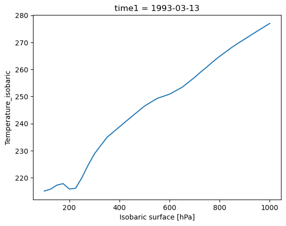
In the figure shown above, Xarray has generated a line plot, which uses the mean temperature profile and the 'isobaric' coordinate variable as axes. In addition, the axis labels and unit information have been read automatically from the DataArray’s metadata.
Customizing the plot
As mentioned above, the .plot() method of Xarray DataArrays uses Matplotlib behind the scenes. Therefore, knowledge of Matplotlib can help you more easily customize plots generated by Xarray.
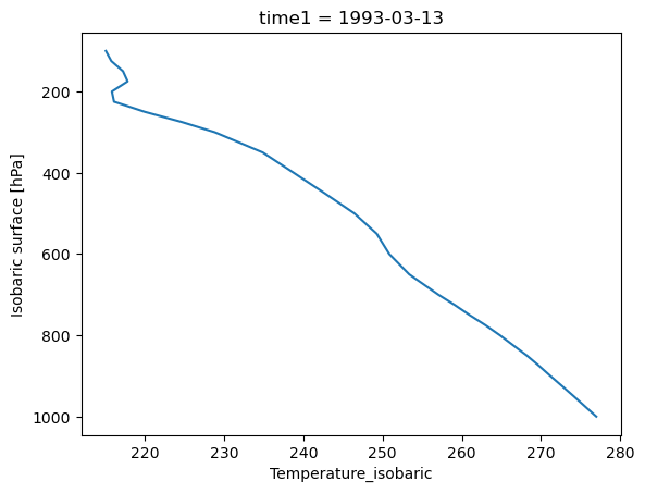
In this example, we need to customize the air temperature profile plot created above. There are two changes that need to be made:
swap the axes, so that the Y (vertical) axis corresponds to isobaric levels
invert the Y axis to match the model of air pressure decreasing at higher altitudes
We can make these changes by adding certain keyword arguments when calling .plot(), as shown below:
prof.plot(y="isobaric1", yincrease=False)
[<matplotlib.lines.Line2D at 0x7f142fafb090>]
Plotting 2-D data
In the previous example, we used .plot() to generate a plot from 1-D data, and the result was a line plot. In this section, we illustrate plotting of 2-D data.
In this example, we illustrate basic plotting of a 2-D array:
temps.sel(isobaric1=1000).plot()
<matplotlib.collections.QuadMesh at 0x7f142fae08d0>
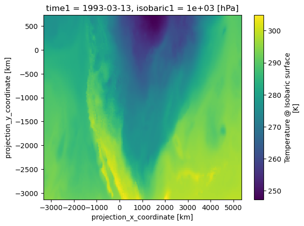
The figure above is generated by Matplotlib’s pcolormesh method, which was automatically called by Xarray’s plot method. This occurred because Xarray recognized that the DataArray object calling the plot method contained two distinct coordinate variables.
The plot generated by the above example is a map of air temperatures over North America, on the 1000 hPa isobaric surface. If a different map projection or added geographic features are needed on this plot, the plot can easily be modified using Cartopy.
Summary
Xarray expands on Pandas’ labeled-data functionality, bringing the usefulness of labeled data operations to N-dimensional data. As such, it has become a central workhorse in the geoscience community for the analysis of gridded datasets. Xarray allows us to open self-describing NetCDF files and make full use of the coordinate axes, labels, units, and other metadata. By making use of labeled coordinates, our code is often easier to write, easier to read, and more robust.
What’s next?
Additional notebooks to appear in this section will describe the following topics in greater detail:
performing arithmetic and broadcasting operations with Xarray data structures
using “group by” operations
remote data access with OPeNDAP
more advanced visualization, including map integration with Cartopy
Resources and references
This tutorial contains content adapted from the material in Unidata’s Python Training.
Most basic questions and issues with Xarray can be resolved with help from the material in the Xarray documentation. Some of the most popular sections of this documentation are listed below:
Another resource you may find useful is this Xarray Tutorial collection, created from content hosted on GitHub.