Introduction to Pandas

---

Overview

1. Introduction to pandas data structures

2. How to slice and dice pandas dataframes and dataseries

3. How to use pandas for exploratory data analysis

Prerequisites

Concepts	Importance	Notes
Python Quickstart	Necessary	Intro to dict
Numpy Basics	Necessary

• Time to learn: 60 minutes

---

Imports

You will often see the nickname pd used as an abbreviation for pandas in the import statement, just like numpy is often imported as np. We also import the DATASETS class from pythia_datasets, which allows us to use example datasets created for Pythia.

import pandas as pd
from pythia_datasets import DATASETS

The pandas DataFrame…

…is a labeled, two-dimensional columnar structure, similar to a table, spreadsheet, or the R data.frame.

The columns that make up our DataFrame can be lists, dictionaries, NumPy arrays, pandas Series, or many other data types not mentioned here. Within these columns, you can have data values of many different data types used in Python and NumPy, including text, numbers, and dates/times. The first column of a DataFrame, shown in the image above in dark gray, is uniquely referred to as an index; this column contains information characterizing each row of our DataFrame. Similar to any other column, the index can label rows by text, numbers, datetime objects, and many other data types. Datetime objects are a quite popular way to label rows.

For our first example using Pandas DataFrames, we start by reading in some data in comma-separated value (.csv) format. We retrieve this dataset from the Pythia DATASETS class (imported at the top of this page); however, the dataset was originally contained within the NCDC teleconnections database. This dataset contains many types of geoscientific data, including El Nino/Southern Oscillation indices. For more information on this dataset, review the description here.

Info

As described above, we are retrieving the datasets for these examples from Project Pythia’s custom library of example data. In order to retrieve datasets from this library, you must use the statement from pythia_datasets import DATASETS. This is shown and described in the Imports section at the top of this page. The fetch() method of the DATASETS class will automatically download the data file specified as a string argument, in this case enso_data.csv, and cache the file locally, assuming the argument corresponds to a valid Pythia example dataset. This is illustrated in the following example.

filepath = DATASETS.fetch('enso_data.csv')

Downloading file 'enso_data.csv' from 'https://github.com/ProjectPythia/pythia-datasets/raw/main/data/enso_data.csv' to '/home/runner/.cache/pythia-datasets'.

Once we have a valid path to a data file that Pandas knows how to read, we can open it, as shown in the following example:

df = pd.read_csv(filepath)

If we print out our DataFrame, it will render as text by default, in a tabular-style ASCII output, as shown in the following example. However, if you are using a Jupyter notebook, there exists a better way to print DataFrames, as described below.

print(df)

       datetime  Nino12  Nino12anom  Nino3  Nino3anom  Nino4  Nino4anom  \
0    1982-01-01   24.29       -0.17  25.87       0.24  28.30       0.00   
1    1982-02-01   25.49       -0.58  26.38       0.01  28.21       0.11   
2    1982-03-01   25.21       -1.31  26.98      -0.16  28.41       0.22   
3    1982-04-01   24.50       -0.97  27.68       0.18  28.92       0.42   
4    1982-05-01   23.97       -0.23  27.79       0.71  29.49       0.70   
..          ...     ...         ...    ...        ...    ...        ...   
467  2020-12-01   22.16       -0.60  24.38      -0.83  27.65      -0.95   
468  2021-01-01   23.89       -0.64  25.06      -0.55  27.10      -1.25   
469  2021-02-01   25.55       -0.66  25.80      -0.57  27.20      -1.00   
470  2021-03-01   26.48       -0.26  26.80      -0.39  27.79      -0.55   
471  2021-04-01   24.89       -0.80  26.96      -0.65  28.47      -0.21   

     Nino34  Nino34anom  
0     26.72        0.15  
1     26.70       -0.02  
2     27.20       -0.02  
3     28.02        0.24  
4     28.54        0.69  
..      ...         ...  
467   25.53       -1.12  
468   25.58       -0.99  
469   25.81       -0.92  
470   26.75       -0.51  
471   27.40       -0.49  

[472 rows x 9 columns]

As described above, there is a better way to print Pandas DataFrames. If you are using a Jupyter notebook, you can run a code cell containing the DataFrame object name, by itself, and it will display a nicely rendered table, as shown below.

df

	datetime	Nino12	Nino12anom	Nino3	Nino3anom	Nino4	Nino4anom	Nino34	Nino34anom
0	1982-01-01	24.29	-0.17	25.87	0.24	28.30	0.00	26.72	0.15
1	1982-02-01	25.49	-0.58	26.38	0.01	28.21	0.11	26.70	-0.02
2	1982-03-01	25.21	-1.31	26.98	-0.16	28.41	0.22	27.20	-0.02
3	1982-04-01	24.50	-0.97	27.68	0.18	28.92	0.42	28.02	0.24
4	1982-05-01	23.97	-0.23	27.79	0.71	29.49	0.70	28.54	0.69
...	...	...	...	...	...	...	...	...	...
467	2020-12-01	22.16	-0.60	24.38	-0.83	27.65	-0.95	25.53	-1.12
468	2021-01-01	23.89	-0.64	25.06	-0.55	27.10	-1.25	25.58	-0.99
469	2021-02-01	25.55	-0.66	25.80	-0.57	27.20	-1.00	25.81	-0.92
470	2021-03-01	26.48	-0.26	26.80	-0.39	27.79	-0.55	26.75	-0.51
471	2021-04-01	24.89	-0.80	26.96	-0.65	28.47	-0.21	27.40	-0.49

472 rows × 9 columns

The DataFrame index, as described above, contains information characterizing rows; each row has a unique ID value, which is displayed in the index column. By default, the IDs for rows in a DataFrame are represented as sequential integers, which start at 0.

df.index

RangeIndex(start=0, stop=472, step=1)

At the moment, the index column of our DataFrame is not very helpful for humans. However, Pandas has clever ways to make index columns more human-readable. The next example demonstrates how to use optional keyword arguments to convert DataFrame index IDs to a human-friendly datetime format.

df = pd.read_csv(filepath, index_col=0, parse_dates=True)

df

	Nino12	Nino12anom	Nino3	Nino3anom	Nino4	Nino4anom	Nino34	Nino34anom
datetime
1982-01-01	24.29	-0.17	25.87	0.24	28.30	0.00	26.72	0.15
1982-02-01	25.49	-0.58	26.38	0.01	28.21	0.11	26.70	-0.02
1982-03-01	25.21	-1.31	26.98	-0.16	28.41	0.22	27.20	-0.02
1982-04-01	24.50	-0.97	27.68	0.18	28.92	0.42	28.02	0.24
1982-05-01	23.97	-0.23	27.79	0.71	29.49	0.70	28.54	0.69
...	...	...	...	...	...	...	...	...
2020-12-01	22.16	-0.60	24.38	-0.83	27.65	-0.95	25.53	-1.12
2021-01-01	23.89	-0.64	25.06	-0.55	27.10	-1.25	25.58	-0.99
2021-02-01	25.55	-0.66	25.80	-0.57	27.20	-1.00	25.81	-0.92
2021-03-01	26.48	-0.26	26.80	-0.39	27.79	-0.55	26.75	-0.51
2021-04-01	24.89	-0.80	26.96	-0.65	28.47	-0.21	27.40	-0.49

472 rows × 8 columns

df.index

DatetimeIndex(['1982-01-01', '1982-02-01', '1982-03-01', '1982-04-01',
               '1982-05-01', '1982-06-01', '1982-07-01', '1982-08-01',
               '1982-09-01', '1982-10-01',
               ...
               '2020-07-01', '2020-08-01', '2020-09-01', '2020-10-01',
               '2020-11-01', '2020-12-01', '2021-01-01', '2021-02-01',
               '2021-03-01', '2021-04-01'],
              dtype='datetime64[ns]', name='datetime', length=472, freq=None)

Each of our data rows is now helpfully labeled by a datetime-object-like index value; this means that we can now easily identify data values not only by named columns, but also by date labels on rows. This is a sneak preview of the DatetimeIndex functionality of Pandas; this functionality enables a large portion of Pandas’ timeseries-related usage. Don’t worry; DatetimeIndex will be discussed in full detail later on this page. In the meantime, let’s look at the columns of data read in from the .csv file:

df.columns

Index(['Nino12', 'Nino12anom', 'Nino3', 'Nino3anom', 'Nino4', 'Nino4anom',
       'Nino34', 'Nino34anom'],
      dtype='object')

The pandas Series…

…is essentially any one of the columns of our DataFrame. A Series also includes the index column from the source DataFrame, in order to provide a label for each value in the Series.

The pandas Series is a fast and capable 1-dimensional array of nearly any data type we could want, and it can behave very similarly to a NumPy ndarray or a Python dict. You can take a look at any of the Series that make up your DataFrame, either by using its column name and the Python dict notation, or by using dot-shorthand with the column name:

df["Nino34"]

datetime
1982-01-01    26.72
1982-02-01    26.70
1982-03-01    27.20
1982-04-01    28.02
1982-05-01    28.54
              ...  
2020-12-01    25.53
2021-01-01    25.58
2021-02-01    25.81
2021-03-01    26.75
2021-04-01    27.40
Name: Nino34, Length: 472, dtype: float64

Tip: You can also use the dot notation illustrated below to specify a column name, but this syntax is mostly provided for convenience. For the most part, this notation is interchangeable with the dictionary notation; however, if the column name is not a valid Python identifier (e.g., it starts with a number or space), you cannot use dot notation.

df.Nino34

datetime
1982-01-01    26.72
1982-02-01    26.70
1982-03-01    27.20
1982-04-01    28.02
1982-05-01    28.54
              ...  
2020-12-01    25.53
2021-01-01    25.58
2021-02-01    25.81
2021-03-01    26.75
2021-04-01    27.40
Name: Nino34, Length: 472, dtype: float64

Slicing and Dicing the DataFrame and Series

In this section, we will expand on topics covered in the previous sections on this page. One of the most important concepts to learn about Pandas is that it allows you to access anything by its associated label, regardless of data organization structure.

Indexing a Series

As a review of previous examples, we’ll start our next example by pulling a Series out of our DataFrame using its column label.

nino34_series = df["Nino34"]

nino34_series

datetime
1982-01-01    26.72
1982-02-01    26.70
1982-03-01    27.20
1982-04-01    28.02
1982-05-01    28.54
              ...  
2020-12-01    25.53
2021-01-01    25.58
2021-02-01    25.81
2021-03-01    26.75
2021-04-01    27.40
Name: Nino34, Length: 472, dtype: float64

You can use syntax similar to that of NumPy ndarrays to index, select, and subset with Pandas Series, as shown in this example:

nino34_series[3]

/tmp/ipykernel_2850/737336773.py:1: FutureWarning: Series.__getitem__ treating keys as positions is deprecated. In a future version, integer keys will always be treated as labels (consistent with DataFrame behavior). To access a value by position, use `ser.iloc[pos]`
  nino34_series[3]

28.02

You can also use labels alongside Python dictionary syntax to perform the same operations:

nino34_series["1982-04-01"]

28.02

You can probably figure out some ways to extend these indexing methods, as shown in the following examples:

nino34_series[0:12]

datetime
1982-01-01    26.72
1982-02-01    26.70
1982-03-01    27.20
1982-04-01    28.02
1982-05-01    28.54
1982-06-01    28.75
1982-07-01    28.10
1982-08-01    27.93
1982-09-01    28.11
1982-10-01    28.64
1982-11-01    28.81
1982-12-01    29.21
Name: Nino34, dtype: float64

Info

Index-based slices are exclusive of the final value, similar to Python’s usual indexing rules.

However, there are many more ways to index a Series. The following example shows a powerful and useful indexing method:

nino34_series["1982-01-01":"1982-12-01"]

datetime
1982-01-01    26.72
1982-02-01    26.70
1982-03-01    27.20
1982-04-01    28.02
1982-05-01    28.54
1982-06-01    28.75
1982-07-01    28.10
1982-08-01    27.93
1982-09-01    28.11
1982-10-01    28.64
1982-11-01    28.81
1982-12-01    29.21
Name: Nino34, dtype: float64

This is an example of label-based slicing. With label-based slicing, Pandas will automatically find a range of values based on the labels you specify.

Info

As opposed to index-based slices, label-based slices are inclusive of the final value.

If you already have some knowledge of xarray, you will quite likely know how to create slice objects by hand. This can also be used in pandas, as shown below. If you are completely unfamiliar with xarray, it will be covered on a later Pythia tutorial page.

nino34_series[slice("1982-01-01", "1982-12-01")]

datetime
1982-01-01    26.72
1982-02-01    26.70
1982-03-01    27.20
1982-04-01    28.02
1982-05-01    28.54
1982-06-01    28.75
1982-07-01    28.10
1982-08-01    27.93
1982-09-01    28.11
1982-10-01    28.64
1982-11-01    28.81
1982-12-01    29.21
Name: Nino34, dtype: float64

Using .iloc and .loc to index

In this section, we introduce ways to access data that are preferred by Pandas over the methods listed above. When accessing by label, it is preferred to use the .loc method, and when accessing by index, the .iloc method is preferred. These methods behave similarly to the notation introduced above, but provide more speed, security, and rigor in your value selection. Using these methods can also help you avoid chained assignment warnings generated by pandas.

nino34_series.iloc[3]

28.02

nino34_series.iloc[0:12]

datetime
1982-01-01    26.72
1982-02-01    26.70
1982-03-01    27.20
1982-04-01    28.02
1982-05-01    28.54
1982-06-01    28.75
1982-07-01    28.10
1982-08-01    27.93
1982-09-01    28.11
1982-10-01    28.64
1982-11-01    28.81
1982-12-01    29.21
Name: Nino34, dtype: float64

nino34_series.loc["1982-04-01"]

28.02

nino34_series.loc["1982-01-01":"1982-12-01"]

datetime
1982-01-01    26.72
1982-02-01    26.70
1982-03-01    27.20
1982-04-01    28.02
1982-05-01    28.54
1982-06-01    28.75
1982-07-01    28.10
1982-08-01    27.93
1982-09-01    28.11
1982-10-01    28.64
1982-11-01    28.81
1982-12-01    29.21
Name: Nino34, dtype: float64

Extending to the DataFrame

These subsetting capabilities can also be used in a full DataFrame; however, if you use the same syntax, there are issues, as shown below:

df["1982-01-01"]

---------------------------------------------------------------------------
KeyError                                  Traceback (most recent call last)
File ~/miniconda3/envs/pythia-book-dev/lib/python3.12/site-packages/pandas/core/indexes/base.py:3805, in Index.get_loc(self, key)
   3804 try:
-> 3805     return self._engine.get_loc(casted_key)
   3806 except KeyError as err:

File index.pyx:167, in pandas._libs.index.IndexEngine.get_loc()

File index.pyx:196, in pandas._libs.index.IndexEngine.get_loc()

File pandas/_libs/hashtable_class_helper.pxi:7081, in pandas._libs.hashtable.PyObjectHashTable.get_item()

File pandas/_libs/hashtable_class_helper.pxi:7089, in pandas._libs.hashtable.PyObjectHashTable.get_item()

KeyError: '1982-01-01'

The above exception was the direct cause of the following exception:

KeyError                                  Traceback (most recent call last)
Cell In[22], line 1
----> 1 df["1982-01-01"]

File ~/miniconda3/envs/pythia-book-dev/lib/python3.12/site-packages/pandas/core/frame.py:4090, in DataFrame.__getitem__(self, key)
   4088 if self.columns.nlevels > 1:
   4089     return self._getitem_multilevel(key)
-> 4090 indexer = self.columns.get_loc(key)
   4091 if is_integer(indexer):
   4092     indexer = [indexer]

File ~/miniconda3/envs/pythia-book-dev/lib/python3.12/site-packages/pandas/core/indexes/base.py:3812, in Index.get_loc(self, key)
   3807     if isinstance(casted_key, slice) or (
   3808         isinstance(casted_key, abc.Iterable)
   3809         and any(isinstance(x, slice) for x in casted_key)
   3810     ):
   3811         raise InvalidIndexError(key)
-> 3812     raise KeyError(key) from err
   3813 except TypeError:
   3814     # If we have a listlike key, _check_indexing_error will raise
   3815     #  InvalidIndexError. Otherwise we fall through and re-raise
   3816     #  the TypeError.
   3817     self._check_indexing_error(key)

KeyError: '1982-01-01'

Danger

Attempting to use Series subsetting with a DataFrame can crash your program. A proper way to subset a DataFrame is shown below.

When indexing a DataFrame, pandas will not assume as readily the intention of your code. In this case, using a row label by itself will not work; with DataFrames, labels are used for identifying columns.

df["Nino34"]

datetime
1982-01-01    26.72
1982-02-01    26.70
1982-03-01    27.20
1982-04-01    28.02
1982-05-01    28.54
              ...  
2020-12-01    25.53
2021-01-01    25.58
2021-02-01    25.81
2021-03-01    26.75
2021-04-01    27.40
Name: Nino34, Length: 472, dtype: float64

As shown below, you also cannot subset columns in a DataFrame using integer indices:

df[0]

---------------------------------------------------------------------------
KeyError                                  Traceback (most recent call last)
File ~/miniconda3/envs/pythia-book-dev/lib/python3.12/site-packages/pandas/core/indexes/base.py:3805, in Index.get_loc(self, key)
   3804 try:
-> 3805     return self._engine.get_loc(casted_key)
   3806 except KeyError as err:

File index.pyx:167, in pandas._libs.index.IndexEngine.get_loc()

File index.pyx:196, in pandas._libs.index.IndexEngine.get_loc()

File pandas/_libs/hashtable_class_helper.pxi:7081, in pandas._libs.hashtable.PyObjectHashTable.get_item()

File pandas/_libs/hashtable_class_helper.pxi:7089, in pandas._libs.hashtable.PyObjectHashTable.get_item()

KeyError: 0

The above exception was the direct cause of the following exception:

KeyError                                  Traceback (most recent call last)
Cell In[24], line 1
----> 1 df[0]

File ~/miniconda3/envs/pythia-book-dev/lib/python3.12/site-packages/pandas/core/frame.py:4090, in DataFrame.__getitem__(self, key)
   4088 if self.columns.nlevels > 1:
   4089     return self._getitem_multilevel(key)
-> 4090 indexer = self.columns.get_loc(key)
   4091 if is_integer(indexer):
   4092     indexer = [indexer]

File ~/miniconda3/envs/pythia-book-dev/lib/python3.12/site-packages/pandas/core/indexes/base.py:3812, in Index.get_loc(self, key)
   3807     if isinstance(casted_key, slice) or (
   3808         isinstance(casted_key, abc.Iterable)
   3809         and any(isinstance(x, slice) for x in casted_key)
   3810     ):
   3811         raise InvalidIndexError(key)
-> 3812     raise KeyError(key) from err
   3813 except TypeError:
   3814     # If we have a listlike key, _check_indexing_error will raise
   3815     #  InvalidIndexError. Otherwise we fall through and re-raise
   3816     #  the TypeError.
   3817     self._check_indexing_error(key)

KeyError: 0

From earlier examples, we know that we can use an index or label with a DataFrame to pull out a column as a Series, and we know that we can use an index or label with a Series to pull out a single value. Therefore, by chaining brackets, we can pull any individual data value out of the DataFrame.

df["Nino34"]["1982-04-01"]

28.02

df["Nino34"][3]

/tmp/ipykernel_2850/541596450.py:1: FutureWarning: Series.__getitem__ treating keys as positions is deprecated. In a future version, integer keys will always be treated as labels (consistent with DataFrame behavior). To access a value by position, use `ser.iloc[pos]`
  df["Nino34"][3]

28.02

However, subsetting data using this chained-bracket technique is not preferred by Pandas. As described above, Pandas prefers us to use the .loc and .iloc methods for subsetting. In addition, these methods provide a clearer, more efficient way to extract specific data from a DataFrame, as illustrated below:

df.loc["1982-04-01", "Nino34"]

28.02

Info

When using this syntax to pull individual data values from a DataFrame, make sure to list the row first, and then the column.

The .loc and .iloc methods also allow us to pull entire rows out of a DataFrame, as shown in these examples:

df.loc["1982-04-01"]

Nino12        24.50
Nino12anom    -0.97
Nino3         27.68
Nino3anom      0.18
Nino4         28.92
Nino4anom      0.42
Nino34        28.02
Nino34anom     0.24
Name: 1982-04-01 00:00:00, dtype: float64

df.loc["1982-01-01":"1982-12-01"]

	Nino12	Nino12anom	Nino3	Nino3anom	Nino4	Nino4anom	Nino34	Nino34anom
datetime
1982-01-01	24.29	-0.17	25.87	0.24	28.30	0.00	26.72	0.15
1982-02-01	25.49	-0.58	26.38	0.01	28.21	0.11	26.70	-0.02
1982-03-01	25.21	-1.31	26.98	-0.16	28.41	0.22	27.20	-0.02
1982-04-01	24.50	-0.97	27.68	0.18	28.92	0.42	28.02	0.24
1982-05-01	23.97	-0.23	27.79	0.71	29.49	0.70	28.54	0.69
1982-06-01	22.89	0.07	27.46	1.03	29.76	0.92	28.75	1.10
1982-07-01	22.47	0.87	26.44	0.82	29.38	0.58	28.10	0.88
1982-08-01	21.75	1.10	26.15	1.16	29.04	0.36	27.93	1.11
1982-09-01	21.80	1.44	26.52	1.67	29.16	0.47	28.11	1.39
1982-10-01	22.94	2.12	27.11	2.19	29.38	0.72	28.64	1.95
1982-11-01	24.59	3.00	27.62	2.64	29.23	0.60	28.81	2.16
1982-12-01	26.13	3.34	28.39	3.25	29.15	0.66	29.21	2.64

df.iloc[3]

Nino12        24.50
Nino12anom    -0.97
Nino3         27.68
Nino3anom      0.18
Nino4         28.92
Nino4anom      0.42
Nino34        28.02
Nino34anom     0.24
Name: 1982-04-01 00:00:00, dtype: float64

df.iloc[0:12]

	Nino12	Nino12anom	Nino3	Nino3anom	Nino4	Nino4anom	Nino34	Nino34anom
datetime
1982-01-01	24.29	-0.17	25.87	0.24	28.30	0.00	26.72	0.15
1982-02-01	25.49	-0.58	26.38	0.01	28.21	0.11	26.70	-0.02
1982-03-01	25.21	-1.31	26.98	-0.16	28.41	0.22	27.20	-0.02
1982-04-01	24.50	-0.97	27.68	0.18	28.92	0.42	28.02	0.24
1982-05-01	23.97	-0.23	27.79	0.71	29.49	0.70	28.54	0.69
1982-06-01	22.89	0.07	27.46	1.03	29.76	0.92	28.75	1.10
1982-07-01	22.47	0.87	26.44	0.82	29.38	0.58	28.10	0.88
1982-08-01	21.75	1.10	26.15	1.16	29.04	0.36	27.93	1.11
1982-09-01	21.80	1.44	26.52	1.67	29.16	0.47	28.11	1.39
1982-10-01	22.94	2.12	27.11	2.19	29.38	0.72	28.64	1.95
1982-11-01	24.59	3.00	27.62	2.64	29.23	0.60	28.81	2.16
1982-12-01	26.13	3.34	28.39	3.25	29.15	0.66	29.21	2.64

In the next example, we illustrate how you can use slices of rows and lists of columns to create a smaller DataFrame out of an existing DataFrame:

df.loc[
    "1982-01-01":"1982-12-01",  # slice of rows
    ["Nino12", "Nino3", "Nino4", "Nino34"],  # list of columns
]

	Nino12	Nino3	Nino4	Nino34
datetime
1982-01-01	24.29	25.87	28.30	26.72
1982-02-01	25.49	26.38	28.21	26.70
1982-03-01	25.21	26.98	28.41	27.20
1982-04-01	24.50	27.68	28.92	28.02
1982-05-01	23.97	27.79	29.49	28.54
1982-06-01	22.89	27.46	29.76	28.75
1982-07-01	22.47	26.44	29.38	28.10
1982-08-01	21.75	26.15	29.04	27.93
1982-09-01	21.80	26.52	29.16	28.11
1982-10-01	22.94	27.11	29.38	28.64
1982-11-01	24.59	27.62	29.23	28.81
1982-12-01	26.13	28.39	29.15	29.21

Info

There are certain limitations to these subsetting techniques. For more information on these limitations, as well as a comparison of DataFrame and Series indexing methods, see the Pandas indexing documentation.

Exploratory Data Analysis

Get a Quick Look at the Beginning/End of your DataFrame

Pandas also gives you a few shortcuts to quickly investigate entire DataFrames. The head method shows the first five rows of a DataFrame, and the tail method shows the last five rows of a DataFrame.

df.head()

	Nino12	Nino12anom	Nino3	Nino3anom	Nino4	Nino4anom	Nino34	Nino34anom
datetime
1982-01-01	24.29	-0.17	25.87	0.24	28.30	0.00	26.72	0.15
1982-02-01	25.49	-0.58	26.38	0.01	28.21	0.11	26.70	-0.02
1982-03-01	25.21	-1.31	26.98	-0.16	28.41	0.22	27.20	-0.02
1982-04-01	24.50	-0.97	27.68	0.18	28.92	0.42	28.02	0.24
1982-05-01	23.97	-0.23	27.79	0.71	29.49	0.70	28.54	0.69

df.tail()

	Nino12	Nino12anom	Nino3	Nino3anom	Nino4	Nino4anom	Nino34	Nino34anom
datetime
2020-12-01	22.16	-0.60	24.38	-0.83	27.65	-0.95	25.53	-1.12
2021-01-01	23.89	-0.64	25.06	-0.55	27.10	-1.25	25.58	-0.99
2021-02-01	25.55	-0.66	25.80	-0.57	27.20	-1.00	25.81	-0.92
2021-03-01	26.48	-0.26	26.80	-0.39	27.79	-0.55	26.75	-0.51
2021-04-01	24.89	-0.80	26.96	-0.65	28.47	-0.21	27.40	-0.49

Quick Plots of Your Data

A good way to explore your data is by making a simple plot. Pandas contains its own plot method; this allows us to plot Pandas series without needing matplotlib. In this example, we plot the Nino34 series of our df DataFrame in this way:

df.Nino34.plot();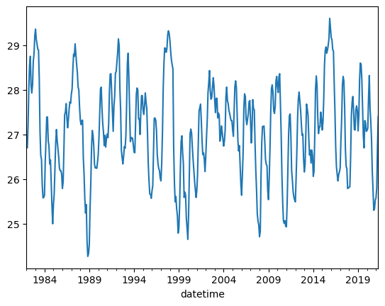

Before, we called .plot(), which generated a single line plot. Line plots can be helpful for understanding some types of data, but there are other types of data that can be better understood with different plot types. For example, if your data values form a distribution, you can better understand them using a histogram plot.

The code for plotting histogram data differs in two ways from the code above for the line plot. First, two series are being used from the DataFrame instead of one. Second, after calling the plot method, we call an additional method called hist, which converts the plot into a histogram.

df[['Nino12', 'Nino34']].plot.hist();

The histogram plot helped us better understand our data; there are clear differences in the distributions. To even better understand this type of data, it may also be helpful to create a box plot. This can be done using the same line of code, with one change: we call the box method instead of hist.

df[['Nino12', 'Nino34']].plot.box();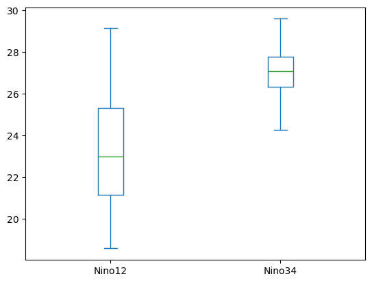

Just like the histogram plot, this box plot indicates a clear difference in the distributions. Using multiple types of plot in this way can be useful for verifying large datasets. The pandas plotting methods are capable of creating many different types of plots. To see how to use the plotting methods to generate each type of plot, please review the pandas plot documentation.

Customize your Plot

The pandas plotting methods are, in fact, wrappers for similar methods in matplotlib. This means that you can customize pandas plots by including keyword arguments to the plotting methods. These keyword arguments, for the most part, are equivalent to their matplotlib counterparts.

df.Nino34.plot(
    color='black',
    linewidth=2,
    xlabel='Year',
    ylabel='ENSO34 Index (degC)',
    figsize=(8, 6),
);

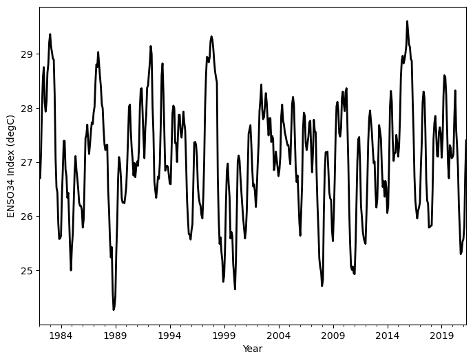
Although plotting data can provide a clear visual picture of data values, sometimes a more quantitative look at data is warranted. As elaborated on in the next section, this can be achieved using the describe method. The describe method is called on the entire DataFrame, and returns various summarized statistics for each column in the DataFrame.

Basic Statistics

We can garner statistics for a DataFrame by using the describe method. When this method is called on a DataFrame, a set of statistics is returned in tabular format. The columns match those of the DataFrame, and the rows indicate different statistics, such as minimum.

df.describe()

	Nino12	Nino12anom	Nino3	Nino3anom	Nino4	Nino4anom	Nino34	Nino34anom
count	472.000000	472.000000	472.000000	472.000000	472.000000	472.000000	472.000000	472.000000
mean	23.209619	0.059725	25.936568	0.039428	28.625064	0.063814	27.076780	0.034894
std	2.431522	1.157590	1.349621	0.965464	0.755422	0.709401	1.063004	0.947936
min	18.570000	-2.100000	23.030000	-2.070000	26.430000	-1.870000	24.270000	-2.380000
25%	21.152500	-0.712500	24.850000	-0.600000	28.140000	-0.430000	26.330000	-0.572500
50%	22.980000	-0.160000	25.885000	-0.115000	28.760000	0.205000	27.100000	0.015000
75%	25.322500	0.515000	26.962500	0.512500	29.190000	0.630000	27.792500	0.565000
max	29.150000	4.620000	29.140000	3.620000	30.300000	1.670000	29.600000	2.950000

You can also view specific statistics using corresponding methods. In this example, we look at the mean values in the entire DataFrame, using the mean method. When such methods are called on the entire DataFrame, a Series is returned. The indices of this Series are the column names in the DataFrame, and the values are the calculated values (in this case, mean values) for the DataFrame columns.

df.mean()

Nino12        23.209619
Nino12anom     0.059725
Nino3         25.936568
Nino3anom      0.039428
Nino4         28.625064
Nino4anom      0.063814
Nino34        27.076780
Nino34anom     0.034894
dtype: float64

If you want a specific statistic for only one column in the DataFrame, pull the column out of the DataFrame with dot notation, then call the statistic function (in this case, mean) on that column, as shown below:

df.Nino34.mean()

27.07677966101695

Subsetting Using the Datetime Column

Slicing is a useful technique for subsetting a DataFrame, but there are also other options that can be equally useful. In this section, some of these additional techniques are covered.

If your DataFrame uses datetime values for indices, you can select data from only one month using df.index.month. In this example, we specify the number 1, which only selects data from January.

# Uses the datetime column
df[df.index.month == 1]

	Nino12	Nino12anom	Nino3	Nino3anom	Nino4	Nino4anom	Nino34	Nino34anom
datetime
1982-01-01	24.29	-0.17	25.87	0.24	28.30	0.00	26.72	0.15
1983-01-01	27.42	2.96	28.92	3.29	29.00	0.70	29.36	2.79
1984-01-01	24.18	-0.28	24.82	-0.81	27.64	-0.66	25.64	-0.93
1985-01-01	23.59	-0.87	24.51	-1.12	27.71	-0.59	25.43	-1.14
1986-01-01	24.61	0.15	24.73	-0.90	28.11	-0.19	25.79	-0.78
1987-01-01	25.30	0.84	26.69	1.06	29.02	0.72	27.91	1.34
1988-01-01	24.64	0.18	26.12	0.49	29.13	0.83	27.32	0.75
1989-01-01	24.09	-0.37	24.15	-1.48	26.54	-1.76	24.53	-2.04
1990-01-01	24.02	-0.44	25.34	-0.29	28.56	0.26	26.55	-0.02
1991-01-01	23.86	-0.60	25.65	0.02	29.00	0.70	27.01	0.44
1992-01-01	24.83	0.37	27.00	1.37	29.06	0.76	28.41	1.84
1993-01-01	24.43	-0.03	25.56	-0.07	28.60	0.30	26.69	0.12
1994-01-01	24.32	-0.14	25.71	0.08	28.47	0.17	26.60	0.03
1995-01-01	25.33	0.87	26.34	0.71	29.20	0.90	27.55	0.98
1996-01-01	23.84	-0.62	24.96	-0.67	27.92	-0.38	25.74	-0.83
1997-01-01	23.67	-0.79	24.70	-0.93	28.41	0.11	25.96	-0.61
1998-01-01	28.22	3.76	28.94	3.31	29.01	0.71	29.10	2.53
1999-01-01	23.73	-0.73	24.41	-1.22	26.59	-1.71	24.90	-1.67
2000-01-01	23.86	-0.60	23.88	-1.75	26.96	-1.34	24.65	-1.92
2001-01-01	23.88	-0.58	24.99	-0.64	27.50	-0.80	25.74	-0.83
2002-01-01	23.64	-0.82	25.09	-0.54	28.81	0.51	26.50	-0.07
2003-01-01	24.38	-0.08	26.38	0.75	29.25	0.95	27.76	1.19
2004-01-01	24.60	0.14	25.92	0.29	28.83	0.53	26.74	0.17
2005-01-01	24.47	0.01	25.89	0.26	29.21	0.91	27.10	0.53
2006-01-01	24.33	-0.13	25.00	-0.63	27.68	-0.62	25.64	-0.93
2007-01-01	24.99	0.53	26.50	0.87	28.93	0.63	27.26	0.69
2008-01-01	23.86	-0.60	24.13	-1.50	26.62	-1.68	24.71	-1.86
2009-01-01	24.42	-0.10	25.03	-0.60	27.42	-0.88	25.54	-1.03
2010-01-01	24.82	0.30	26.63	1.00	29.51	1.21	28.07	1.50
2011-01-01	24.08	-0.44	24.31	-1.32	26.72	-1.58	24.93	-1.64
2012-01-01	23.88	-0.64	24.90	-0.73	27.09	-1.21	25.49	-1.08
2013-01-01	24.00	-0.52	25.06	-0.57	28.28	-0.02	26.16	-0.41
2014-01-01	24.79	0.27	25.26	-0.37	28.14	-0.17	26.06	-0.51
2015-01-01	24.13	-0.39	25.99	0.36	29.16	0.86	27.10	0.53
2016-01-01	25.93	1.41	28.21	2.58	29.65	1.35	29.17	2.60
2017-01-01	25.75	1.23	25.61	-0.02	28.18	-0.12	26.25	-0.32
2018-01-01	23.71	-0.81	24.48	-1.14	28.03	-0.27	25.82	-0.75
2019-01-01	25.10	0.57	26.17	0.55	29.00	0.65	27.08	0.52
2020-01-01	24.55	0.02	25.81	0.20	29.28	0.93	27.09	0.53
2021-01-01	23.89	-0.64	25.06	-0.55	27.10	-1.25	25.58	-0.99

This example shows how to create a new column containing the month portion of the datetime index for each data row. The value returned by df.index.month is used to obtain the data for this new column:

df['month'] = df.index.month

This next example illustrates how to use the new month column to calculate average monthly values over the other data columns. First, we use the groupby method to group the other columns by the month. Second, we take the average (mean) to obtain the monthly averages. Finally, we plot the resulting data as a line plot by simply calling plot().

df.groupby('month').mean().plot();

Investigating Extreme Values

If you need to search for rows that meet a specific criterion, you can use conditional indexing. In this example, we search for rows where the Nino34 anomaly value (Nino34anom) is greater than 2:

df[df.Nino34anom > 2]

	Nino12	Nino12anom	Nino3	Nino3anom	Nino4	Nino4anom	Nino34	Nino34anom	month
datetime
1982-11-01	24.59	3.00	27.62	2.64	29.23	0.60	28.81	2.16	11
1982-12-01	26.13	3.34	28.39	3.25	29.15	0.66	29.21	2.64	12
1983-01-01	27.42	2.96	28.92	3.29	29.00	0.70	29.36	2.79	1
1983-02-01	28.09	2.02	28.92	2.55	28.79	0.69	29.13	2.41	2
1997-08-01	24.80	4.15	27.84	2.85	29.26	0.58	28.84	2.02	8
1997-09-01	24.40	4.04	27.84	2.99	29.32	0.63	28.93	2.21	9
1997-10-01	24.58	3.76	28.17	3.25	29.32	0.66	29.23	2.54	10
1997-11-01	25.63	4.04	28.55	3.57	29.49	0.86	29.32	2.67	11
1997-12-01	26.92	4.13	28.76	3.62	29.32	0.83	29.26	2.69	12
1998-01-01	28.22	3.76	28.94	3.31	29.01	0.71	29.10	2.53	1
1998-02-01	28.98	2.91	28.93	2.56	28.87	0.77	28.86	2.14	2
2015-08-01	22.88	2.24	27.33	2.34	29.66	0.98	28.89	2.07	8
2015-09-01	22.91	2.57	27.48	2.63	29.73	1.04	29.00	2.28	9
2015-10-01	23.31	2.52	27.58	2.66	29.79	1.12	29.15	2.46	10
2015-11-01	23.83	2.24	27.91	2.93	30.30	1.67	29.60	2.95	11
2015-12-01	25.01	2.19	27.99	2.85	30.11	1.63	29.39	2.82	12
2016-01-01	25.93	1.41	28.21	2.58	29.65	1.35	29.17	2.60	1
2016-02-01	26.81	0.67	28.36	1.99	29.55	1.45	29.12	2.40	2

This example shows how to use the sort_values method on a DataFrame. This method sorts values in a DataFrame by the column specified as an argument.

df.sort_values('Nino34anom')

	Nino12	Nino12anom	Nino3	Nino3anom	Nino4	Nino4anom	Nino34	Nino34anom	month
datetime
1988-11-01	20.55	-1.04	23.03	-1.95	26.76	-1.87	24.27	-2.38	11
1988-12-01	21.80	-0.99	23.07	-2.07	26.75	-1.74	24.33	-2.24	12
1988-10-01	19.50	-1.32	23.17	-1.75	27.06	-1.60	24.62	-2.07	10
1989-01-01	24.09	-0.37	24.15	-1.48	26.54	-1.76	24.53	-2.04	1
2000-01-01	23.86	-0.60	23.88	-1.75	26.96	-1.34	24.65	-1.92	1
...	...	...	...	...	...	...	...	...	...
1997-11-01	25.63	4.04	28.55	3.57	29.49	0.86	29.32	2.67	11
1997-12-01	26.92	4.13	28.76	3.62	29.32	0.83	29.26	2.69	12
1983-01-01	27.42	2.96	28.92	3.29	29.00	0.70	29.36	2.79	1
2015-12-01	25.01	2.19	27.99	2.85	30.11	1.63	29.39	2.82	12
2015-11-01	23.83	2.24	27.91	2.93	30.30	1.67	29.60	2.95	11

472 rows × 9 columns

You can also reverse the ordering of the sort by specifying the ascending keyword argument as False:

df.sort_values('Nino34anom', ascending=False)

	Nino12	Nino12anom	Nino3	Nino3anom	Nino4	Nino4anom	Nino34	Nino34anom	month
datetime
2015-11-01	23.83	2.24	27.91	2.93	30.30	1.67	29.60	2.95	11
2015-12-01	25.01	2.19	27.99	2.85	30.11	1.63	29.39	2.82	12
1983-01-01	27.42	2.96	28.92	3.29	29.00	0.70	29.36	2.79	1
1997-12-01	26.92	4.13	28.76	3.62	29.32	0.83	29.26	2.69	12
1997-11-01	25.63	4.04	28.55	3.57	29.49	0.86	29.32	2.67	11
...	...	...	...	...	...	...	...	...	...
2000-01-01	23.86	-0.60	23.88	-1.75	26.96	-1.34	24.65	-1.92	1
1989-01-01	24.09	-0.37	24.15	-1.48	26.54	-1.76	24.53	-2.04	1
1988-10-01	19.50	-1.32	23.17	-1.75	27.06	-1.60	24.62	-2.07	10
1988-12-01	21.80	-0.99	23.07	-2.07	26.75	-1.74	24.33	-2.24	12
1988-11-01	20.55	-1.04	23.03	-1.95	26.76	-1.87	24.27	-2.38	11

472 rows × 9 columns

Resampling

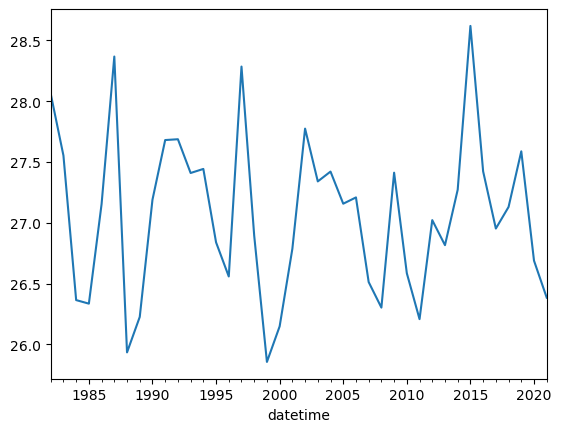
In these examples, we illustrate a process known as resampling. Using resampling, you can change the frequency of index data values, reducing so-called ‘noise’ in a data plot. This is especially useful when working with timeseries data; plots can be equally effective with resampled data in these cases. The resampling performed in these examples converts monthly values to yearly averages. This is performed by passing the value ‘1Y’ to the resample method.

df.Nino34.plot();

df.Nino34.resample('1Y').mean().plot();

/tmp/ipykernel_2850/233158901.py:1: FutureWarning: 'Y' is deprecated and will be removed in a future version, please use 'YE' instead.
  df.Nino34.resample('1Y').mean().plot();

Applying operations to a DataFrame

One of the most commonly used features in Pandas is the performing of calculations to multiple data values in a DataFrame simultaneously. Let’s first look at a familiar concept: a function that converts single values. The following example uses such a function to convert temperature values from degrees Celsius to Kelvin.

def convert_degc_to_kelvin(temperature_degc):
    """
    Converts from degrees celsius to Kelvin
    """

    return temperature_degc + 273.15

# Convert a single value
convert_degc_to_kelvin(0)

273.15

The following examples instead illustrate a new concept: using such functions with DataFrames and Series. For the first example, we start by creating a Series; in order to do so, we subset the DataFrame by the Nino34 column. This has already been done earlier in this page; we do not need to create this Series again. We are using this particular Series for a reason: the data values are in degrees Celsius.

nino34_series

datetime
1982-01-01    26.72
1982-02-01    26.70
1982-03-01    27.20
1982-04-01    28.02
1982-05-01    28.54
              ...  
2020-12-01    25.53
2021-01-01    25.58
2021-02-01    25.81
2021-03-01    26.75
2021-04-01    27.40
Name: Nino34, Length: 472, dtype: float64

Here, we look at a portion of an existing DataFrame column. Notice that this column portion is a Pandas Series.

type(df.Nino12[0:10])

pandas.core.series.Series

As shown in the following example, each Pandas Series contains a representation of its data in numpy format. Therefore, it is possible to convert a Pandas Series into a numpy array; this is done using the .values method:

type(df.Nino12.values[0:10])

numpy.ndarray

This example illustrates how to use the temperature-conversion function defined above on a Series object. Just as calling the function with a single value returns a single value, calling the function on a Series object returns another Series object. The function performs the temperature conversion on each data value in the Series, and returns a Series with all values converted.

convert_degc_to_kelvin(nino34_series)

datetime
1982-01-01    299.87
1982-02-01    299.85
1982-03-01    300.35
1982-04-01    301.17
1982-05-01    301.69
               ...  
2020-12-01    298.68
2021-01-01    298.73
2021-02-01    298.96
2021-03-01    299.90
2021-04-01    300.55
Name: Nino34, Length: 472, dtype: float64

If we call the .values method on the Series passed to the function, the Series is converted to a numpy array, as described above. The function then converts each value in the numpy array, and returns a new numpy array with all values sorted.

Warning

It is recommended to only convert Series to NumPy arrays when necessary; doing so removes the label information that enables much of the Pandas core functionality.

convert_degc_to_kelvin(nino34_series.values)

array([299.87, 299.85, 300.35, 301.17, 301.69, 301.9 , 301.25, 301.08,
       301.26, 301.79, 301.96, 302.36, 302.51, 302.28, 302.18, 302.06,
       302.04, 301.39, 300.22, 299.68, 299.59, 299.02, 298.73, 298.74,
       298.79, 299.54, 300.01, 300.54, 300.54, 300.01, 299.89, 299.49,
       299.58, 299.08, 298.56, 298.15, 298.58, 298.82, 299.38, 299.95,
       300.26, 300.01, 299.84, 299.65, 299.4 , 299.34, 299.34, 299.26,
       298.94, 299.09, 299.8 , 300.59, 300.65, 300.84, 300.52, 300.3 ,
       300.48, 300.72, 300.88, 300.85, 301.06, 301.17, 301.62, 301.95,
       301.9 , 302.18, 301.95, 301.73, 301.54, 301.22, 301.14, 300.75,
       300.47, 300.37, 300.46, 300.47, 299.63, 299.26, 298.72, 298.39,
       298.58, 297.77, 297.42, 297.48, 297.68, 298.48, 299.05, 299.84,
       300.24, 300.13, 299.89, 299.48, 299.4 , 299.41, 299.39, 299.53,
       299.7 , 300.1 , 300.61, 301.17, 301.21, 300.73, 300.4 , 300.2 ,
       299.9 , 300.13, 299.87, 300.06, 300.16, 300.08, 300.4 , 301.13,
       301.5 , 301.51, 301.07, 300.59, 300.22, 300.78, 301.01, 301.52,
       301.56, 301.78, 301.98, 302.29, 302.14, 301.17, 300.68, 299.79,
       299.63, 299.49, 299.66, 299.88, 299.84, 300.12, 300.81, 301.74,
       301.97, 301.43, 300.7 , 299.99, 300.07, 300.08, 300.06, 299.91,
       299.75, 299.74, 300.42, 301.05, 301.19, 301.14, 300.5 , 300.5 ,
       300.15, 300.64, 301.02, 301.02, 300.7 , 300.6 , 300.78, 301.08,
       300.88, 300.74, 300.16, 299.48, 299.11, 298.82, 298.81, 298.72,
       298.89, 299.  , 299.77, 300.51, 300.52, 300.47, 300.24, 299.71,
       299.5 , 299.39, 299.34, 299.17, 299.11, 299.51, 300.18, 301.18,
       301.75, 302.09, 302.07, 301.99, 302.08, 302.38, 302.47, 302.41,
       302.25, 302.01, 301.82, 301.71, 301.62, 299.87, 299.09, 298.64,
       298.76, 298.49, 298.33, 297.94, 298.05, 298.56, 299.4 , 299.99,
       300.12, 299.75, 299.5 , 298.74, 298.86, 298.79, 298.27, 298.05,
       297.8 , 298.34, 299.23, 300.16, 300.27, 300.18, 299.87, 299.6 ,
       299.36, 299.11, 298.93, 298.74, 298.89, 299.26, 299.99, 300.67,
       300.75, 300.83, 300.47, 300.02, 299.7 , 299.74, 299.6 , 299.32,
       299.65, 300.1 , 300.47, 301.09, 301.3 , 301.58, 301.13, 300.94,
       300.98, 301.2 , 301.42, 301.24, 300.91, 300.64, 300.96, 300.96,
       300.52, 300.63, 300.58, 300.  , 300.11, 300.34, 300.2 , 300.04,
       299.89, 300.01, 300.25, 300.99, 301.21, 300.91, 300.84, 300.69,
       300.62, 300.53, 300.46, 300.46, 300.25, 300.11, 300.7 , 301.22,
       301.35, 301.2 , 300.62, 300.03, 299.78, 299.9 , 299.49, 299.04,
       298.79, 299.23, 299.72, 300.74, 301.06, 301.  , 300.5 , 300.37,
       300.49, 300.62, 300.88, 300.91, 300.41, 299.96, 300.33, 300.93,
       300.72, 300.7 , 299.94, 299.35, 298.92, 298.37, 298.21, 298.12,
       297.86, 297.98, 299.22, 299.98, 300.33, 300.32, 300.34, 300.  ,
       299.59, 299.48, 299.45, 298.89, 298.69, 299.19, 299.82, 300.65,
       301.18, 301.26, 301.09, 300.68, 300.62, 300.78, 301.34, 301.45,
       301.22, 301.09, 301.44, 301.51, 300.83, 300.15, 299.24, 298.65,
       298.22, 298.16, 298.22, 298.1 , 298.08, 298.61, 299.38, 300.17,
       300.57, 300.61, 300.11, 299.34, 299.13, 298.87, 298.75, 298.68,
       298.64, 299.18, 299.78, 300.53, 300.95, 301.1 , 300.9 , 300.7 ,
       300.39, 300.13, 300.16, 299.61, 299.31, 299.47, 300.15, 300.83,
       300.72, 300.58, 300.06, 299.69, 299.8 , 299.51, 299.8 , 299.68,
       299.21, 299.33, 300.14, 301.16, 301.46, 301.26, 300.55, 300.17,
       300.32, 300.32, 300.65, 300.5 , 300.25, 300.44, 300.94, 301.71,
       302.03, 302.11, 301.97, 302.04, 302.15, 302.3 , 302.75, 302.54,
       302.32, 302.27, 302.05, 302.02, 301.3 , 300.68, 299.88, 299.43,
       299.26, 299.11, 299.25, 299.31, 299.4 , 300.02, 300.49, 301.25,
       301.45, 301.34, 300.76, 299.82, 299.44, 299.38, 298.94, 298.95,
       298.97, 298.98, 299.63, 300.57, 300.87, 301.  , 300.67, 300.26,
       300.25, 300.7 , 300.79, 300.68, 300.23, 300.56, 301.37, 301.75,
       301.72, 301.39, 300.78, 300.12, 299.85, 300.46, 300.41, 300.22,
       300.24, 300.29, 300.97, 301.47, 300.74, 300.45, 300.04, 299.33,
       298.92, 298.45, 298.49, 298.68, 298.73, 298.96, 299.9 , 300.55])

As described above, when our temperature-conversion function accepts a Series as an argument, it returns a Series. We can directly assign this returned Series to a new column in our DataFrame, as shown below:

df['Nino34_degK'] = convert_degc_to_kelvin(nino34_series)

df.Nino34_degK

datetime
1982-01-01    299.87
1982-02-01    299.85
1982-03-01    300.35
1982-04-01    301.17
1982-05-01    301.69
               ...  
2020-12-01    298.68
2021-01-01    298.73
2021-02-01    298.96
2021-03-01    299.90
2021-04-01    300.55
Name: Nino34_degK, Length: 472, dtype: float64

In this final example, we demonstrate the use of the to_csv method to save a DataFrame as a .csv file. This example also demonstrates the read_csv method, which reads .csv files into Pandas DataFrames.

df.to_csv('nino_analyzed_output.csv')

pd.read_csv('nino_analyzed_output.csv', index_col=0, parse_dates=True)

	Nino12	Nino12anom	Nino3	Nino3anom	Nino4	Nino4anom	Nino34	Nino34anom	month	Nino34_degK
datetime
1982-01-01	24.29	-0.17	25.87	0.24	28.30	0.00	26.72	0.15	1	299.87
1982-02-01	25.49	-0.58	26.38	0.01	28.21	0.11	26.70	-0.02	2	299.85
1982-03-01	25.21	-1.31	26.98	-0.16	28.41	0.22	27.20	-0.02	3	300.35
1982-04-01	24.50	-0.97	27.68	0.18	28.92	0.42	28.02	0.24	4	301.17
1982-05-01	23.97	-0.23	27.79	0.71	29.49	0.70	28.54	0.69	5	301.69
...	...	...	...	...	...	...	...	...	...	...
2020-12-01	22.16	-0.60	24.38	-0.83	27.65	-0.95	25.53	-1.12	12	298.68
2021-01-01	23.89	-0.64	25.06	-0.55	27.10	-1.25	25.58	-0.99	1	298.73
2021-02-01	25.55	-0.66	25.80	-0.57	27.20	-1.00	25.81	-0.92	2	298.96
2021-03-01	26.48	-0.26	26.80	-0.39	27.79	-0.55	26.75	-0.51	3	299.90
2021-04-01	24.89	-0.80	26.96	-0.65	28.47	-0.21	27.40	-0.49	4	300.55

472 rows × 10 columns

---

Summary

• Pandas is a very powerful tool for working with tabular (i.e., spreadsheet-style) data

• There are multiple ways of subsetting your pandas dataframe or series

• Pandas allows you to refer to subsets of data by label, which generally makes code more readable and more robust

• Pandas can be helpful for exploratory data analysis, including plotting and basic statistics

• One can apply calculations to pandas dataframes and save the output via csv files

What’s Next?

In the next notebook, we will look more into using pandas for more in-depth data analysis.

Resources and References

1. NOAA NCDC ENSO Dataset Used in this Example

2. Getting Started with Pandas

3. Pandas User Guide