
The scientific Python package known as Dask provides Dask Arrays: parallel, larger-than-memory, n-dimensional arrays that make use of blocked algorithms. They are analogous to Numpy arrays, but are distributed. These terms are defined below:
- Parallel code uses many or all of the cores on the computer running the code.
- Larger-than-memory refers to algorithms that break up data arrays into small pieces, operate on these pieces in an optimized fashion, and stream data from a storage device. This allows a user or programmer to work with datasets of a size larger than the available memory.
- A blocked algorithm speeds up large computations by converting them into a series of smaller computations.
In this tutorial, we cover the use of Xarray to wrap Dask arrays. By using Dask arrays instead of Numpy arrays in Xarray data objects, it becomes possible to execute analysis code in parallel with much less code and effort.
Learning Objectives
- Learn the distinction between eager and lazy execution, and performing both types of execution with Xarray
- Understand key features of Dask Arrays
- Learn to perform operations with Dask Arrays in similar ways to performing operations with NumPy arrays
- Understand the use of Xarray
DataArraysandDatasetsas “Dask collections”, and the use of top-level Dask functions such asdask.visualize()on such collections - Understand the ability to use Dask transparently in all built-in Xarray operations
Prerequisites
| Concepts | Importance | Notes |
|---|---|---|
| Introduction to NumPy | Necessary | Familiarity with Data Arrays |
| Introduction to Xarray | Necessary | Familiarity with Xarray Data Structures |
- Time to learn: 30-40 minutes
Imports
For this tutorial, as we are working with Dask, there are a number of Dask packages that must be imported. Also, this is technically an Xarray tutorial, so Xarray and NumPy must also be imported. Finally, the Pythia datasets package is imported, allowing access to the Project Pythia example data library.
import dask
import dask.array as da
import numpy as np
import xarray as xr
from dask.diagnostics import ProgressBar
from dask.utils import format_bytes
from pythia_datasets import DATASETS
/home/runner/micromamba/envs/pythia-book-dev/lib/python3.13/site-packages/pythia_datasets/__init__.py:4: UserWarning: pkg_resources is deprecated as an API. See https://setuptools.pypa.io/en/latest/pkg_resources.html. The pkg_resources package is slated for removal as early as 2025-11-30. Refrain from using this package or pin to Setuptools<81.
from pkg_resources import DistributionNotFound, get_distribution
Blocked algorithms
As described above, the definition of “blocked algorithm” is an algorithm that replaces a large operation with many small operations. In the case of datasets, this means that a blocked algorithm separates a dataset into chunks, and performs an operation on each.
As an example of how blocked algorithms work, consider a dataset containing a billion numbers, and assume that the sum of the numbers is needed. Using a non-blocked algorithm, all of the numbers are added in one operation, which is extremely inefficient. However, by using a blocked algorithm, the dataset is broken into chunks. (For the purposes of this example, assume that 1,000 chunks are created, with 1,000,000 numbers each.) The sum of the numbers in each chunk is taken, most likely in parallel, and then each of those sums are summed to obtain the final result.
By using blocked algorithms, we achieve the result, in this case one sum of one billion numbers, through the results of many smaller operations, in this case one thousand sums of one million numbers each. (Also note that each of the one thousand sums must then be summed, making the total number of sums 1,001.) This allows for a much greater degree of parallelism, potentially speeding up the code execution dramatically.
dask.array contains these algorithms
The main object type used in Dask is dask.array, which implements a subset of the ndarray (NumPy array) interface. However, unlike ndarray, dask.array uses blocked algorithms, which break up the array into smaller arrays, as described above. This allows for the execution of computations on arrays larger than memory, by using parallelism to divide the computation among multiple cores. Dask manages and coordinates blocked algorithms for any given computation by using Dask graphs, which lay out in detail the steps Dask takes to solve a problem. In addition, dask.array objects, known as Dask Arrays, are lazy; in other words, any computation performed on them is delayed until a specific method is called.
Create a dask.array object
As stated earlier, Dask Arrays are loosely based on NumPy arrays. In the next set of examples, we illustrate the main differences between Dask Arrays and NumPy arrays. In order to illustrate the differences, we must have both a Dask Array object and a NumPy array object. Therefore, this first example creates a 3-D NumPy array of random data:
shape = (600, 200, 200)
arr = np.random.random(shape)
arr
array([[[9.19585856e-02, 9.37414693e-01, 3.23310420e-01, ...,
6.55013311e-01, 6.68111000e-01, 6.62606979e-01],
[5.13448169e-01, 4.63597538e-01, 5.21526773e-01, ...,
2.96512476e-01, 3.62261180e-02, 1.15177151e-01],
[3.77628403e-01, 6.23402762e-01, 1.63185306e-01, ...,
3.57715072e-01, 1.59953032e-01, 1.51217063e-01],
...,
[1.97202803e-01, 1.97401056e-01, 1.96507311e-01, ...,
9.18560231e-01, 2.82970005e-03, 4.11919283e-01],
[2.31897415e-02, 9.56553757e-01, 2.62897617e-02, ...,
1.27332127e-01, 2.01379024e-01, 3.05449948e-01],
[7.46528815e-02, 1.15725946e-01, 8.65624093e-01, ...,
5.44574635e-01, 7.43041852e-01, 6.32926873e-01]],
[[5.47157159e-01, 3.24902850e-01, 2.09473847e-01, ...,
5.98965262e-01, 1.52680126e-03, 8.62380017e-01],
[4.84544964e-01, 2.16263026e-02, 1.73496626e-01, ...,
5.75570020e-01, 2.67766131e-01, 3.50828779e-01],
[3.13393135e-01, 9.24812274e-02, 2.45574391e-01, ...,
4.78293513e-01, 8.71801183e-01, 3.83732299e-01],
...,
[2.26230126e-01, 3.51420349e-01, 3.90601437e-01, ...,
4.98169104e-01, 9.42044961e-01, 9.10098965e-01],
[6.54244553e-04, 4.95013163e-01, 1.98812996e-01, ...,
3.17746494e-01, 4.54719598e-01, 4.79681139e-01],
[7.09690956e-01, 4.96592561e-01, 9.12664779e-01, ...,
7.92971947e-01, 9.89796953e-01, 3.87204128e-01]],
[[3.82661902e-01, 3.35460944e-01, 5.91400618e-01, ...,
2.91954511e-01, 8.51598199e-02, 4.03251475e-01],
[7.59685194e-01, 3.50939149e-01, 8.22256364e-01, ...,
2.95080753e-01, 2.44870911e-01, 1.23945470e-01],
[5.36105375e-01, 2.55187904e-01, 4.98151353e-02, ...,
9.78369497e-01, 2.83278847e-01, 3.03527598e-01],
...,
[7.46089732e-01, 6.60934901e-01, 5.50816329e-02, ...,
9.55656207e-01, 8.66463299e-01, 4.06068372e-02],
[1.41071362e-01, 1.93880209e-01, 6.86896911e-01, ...,
3.22246129e-01, 1.36674593e-01, 8.79911625e-01],
[7.96588862e-01, 3.44639044e-01, 7.55527315e-01, ...,
7.76137508e-01, 8.70208436e-01, 9.53243108e-01]],
...,
[[4.97588077e-01, 7.75739307e-01, 9.48270193e-01, ...,
2.98700644e-01, 5.98727037e-01, 6.13542864e-01],
[5.87907764e-01, 4.70909888e-01, 9.35917972e-01, ...,
7.03671399e-01, 4.97547749e-01, 4.12723857e-01],
[5.12365818e-01, 2.55701108e-01, 2.93912960e-01, ...,
5.41929202e-01, 5.19722192e-01, 4.37579583e-01],
...,
[5.81751250e-01, 2.19113654e-01, 7.90092054e-02, ...,
3.21587297e-01, 6.26850783e-01, 2.39507310e-01],
[6.02504075e-01, 5.35953839e-01, 5.96869782e-01, ...,
1.08900237e-01, 4.88966850e-03, 1.09308727e-01],
[6.33233966e-01, 6.53409125e-01, 4.41298873e-01, ...,
1.98836260e-01, 3.56847176e-01, 8.39096047e-01]],
[[9.32661775e-01, 4.13652128e-01, 4.33830684e-02, ...,
9.61748586e-01, 7.67494524e-01, 7.25343445e-01],
[8.06078516e-01, 8.57508052e-01, 6.31283535e-01, ...,
9.76463856e-01, 7.29044019e-02, 3.79432921e-01],
[9.34215037e-01, 9.36282650e-01, 2.76555574e-01, ...,
8.82108737e-01, 5.98137462e-01, 1.02276318e-01],
...,
[3.03372018e-01, 2.59428531e-01, 9.58774014e-01, ...,
3.90018513e-01, 3.19952872e-01, 1.18522861e-01],
[2.85064808e-01, 8.50859558e-01, 7.16594492e-01, ...,
2.19919923e-01, 5.97289529e-01, 3.90229754e-01],
[6.52720488e-02, 4.25302320e-01, 2.91745880e-01, ...,
2.19402945e-01, 7.34035066e-02, 6.48962845e-01]],
[[5.24874714e-01, 1.09305920e-01, 7.94031513e-01, ...,
3.51585578e-01, 3.22501376e-01, 3.53986180e-01],
[4.59765310e-01, 8.46257256e-01, 9.64646700e-01, ...,
8.97088635e-01, 2.37302984e-01, 6.84658170e-01],
[3.36889301e-01, 3.39949819e-01, 3.85922492e-01, ...,
7.72366015e-01, 6.20420231e-01, 3.82104254e-01],
...,
[2.52861932e-01, 4.42274163e-01, 9.56896325e-02, ...,
3.47069093e-01, 2.37888144e-01, 4.65610032e-01],
[6.52403370e-01, 9.05042571e-02, 2.16394766e-01, ...,
9.07552018e-01, 3.91855454e-01, 5.47947826e-01],
[5.73415073e-01, 4.04976808e-01, 8.86016731e-01, ...,
8.80169176e-01, 7.12170689e-01, 3.71440268e-01]]],
shape=(600, 200, 200))format_bytes(arr.nbytes)'183.11 MiB'As shown above, this NumPy array contains about 183 MB of data.
As stated above, we must also create a Dask Array. This next example creates a Dask Array with the same dimension sizes as the existing NumPy array:
darr = da.random.random(shape, chunks=(300, 100, 200))By specifying values to the chunks keyword argument, we can specify the array pieces that Dask’s blocked algorithms break the array into; in this case, we specify (300, 100, 200).
If you are viewing this page as a Jupyter Notebook, the next Jupyter cell will produce a rich information graphic giving in-depth details about the array and each individual chunk.
darrThe above graphic contains a symbolic representation of the array, including shape, dtype, and chunksize. (Your view may be different, depending on how you are accessing this page.) Notice that there is no data shown for this array; this is because Dask Arrays are lazy, as described above. Before we call a compute method for this array, we first illustrate the structure of a Dask graph. In this example, we show the Dask graph by calling .visualize() on the array:
darr.visualize()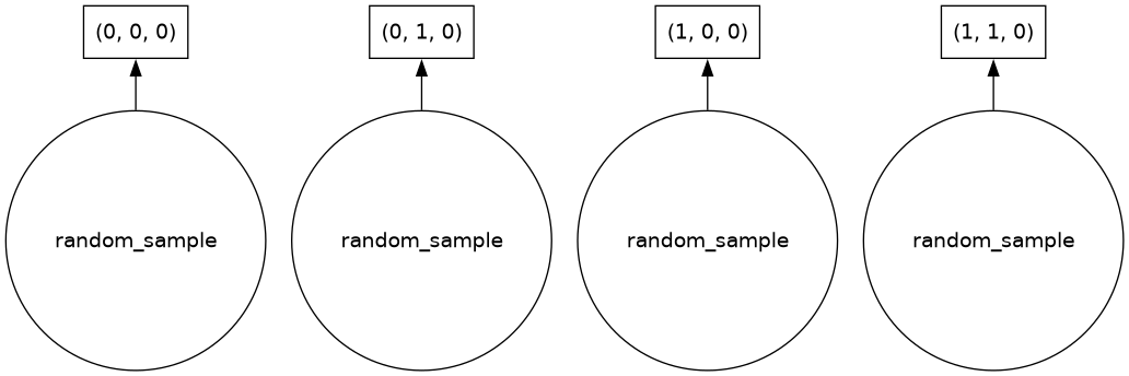
As shown in the above Dask graph, our array has four chunks, each one created by a call to NumPy’s “random” method (np.random.random). These chunks are concatenated into a single array after the calculation is performed.
Manipulate a dask.array object as you would a numpy array
We can perform computations on the Dask Array created above in a similar fashion to NumPy arrays. These computations include arithmetic, slicing, and reductions, among others.
Although the code for performing these computations is similar between NumPy arrays and Dask Arrays, the process by which they are performed is quite different. For example, it is possible to call sum() on both a NumPy array and a Dask Array; however, these two sum() calls are definitely not the same, as shown below.
What’s the difference?
When sum() is called on a Dask Array, the computation is not performed; instead, an expression of the computation is built. The sum() computation, as well as any other computation methods called on the same Dask Array, are not performed until a specific method (known as a compute method) is called on the array. (This is known as lazy execution.) On the other hand, calling sum() on a NumPy array performs the calculation immediately; this is known as eager execution.
Why the difference?
As described earlier, a Dask Array is divided into chunks. Any computations run on the Dask Array run on each chunk individually. If the result of the computation is obtained before the computation runs through all of the chunks, Dask can stop the computation to save CPU time and memory resources.
This example illustrates calling sum() on a Dask Array; it also includes a demonstration of lazy execution, as well as another Dask graph display:
total = darr.sum()
totaltotal.visualize()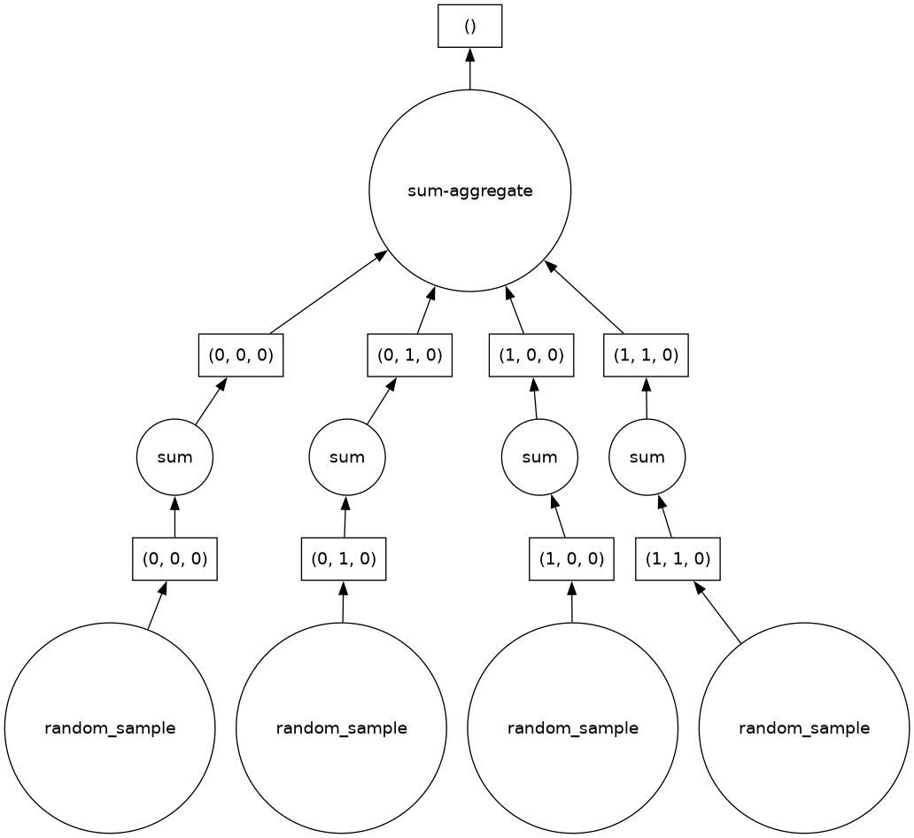
Compute the result
As described above, Dask Array objects make use of lazy execution. Therefore, operations performed on a Dask Array wait to execute until a compute method is called. As more operations are queued in this way, the Dask Array’s Dask graph increases in complexity, reflecting the steps Dask will take to perform all of the queued operations.
In this example, we call a compute method, simply called .compute(), to run on the Dask Array all of the stored computations:
%%time
total.compute()
CPU times: user 395 ms, sys: 54.2 ms, total: 449 ms
Wall time: 1.06 s
np.float64(11997240.38278617)Exercise with dask.arrays
In this section of the page, the examples are hands-on exercises pertaining to Dask Arrays. If these exercises are not interesting to you, this section can be used strictly as examples regardless of how the page is viewed. However, if you wish to participate in the exercises, make sure that you are viewing this page as a Jupyter Notebook.
For the first exercise, modify the chunk size or shape of the Dask Array created earlier. Call .sum() on the modified Dask Array, and visualize the Dask graph to view the changes.
da.random.random(shape, chunks=(50, 200, 400)).sum().visualize()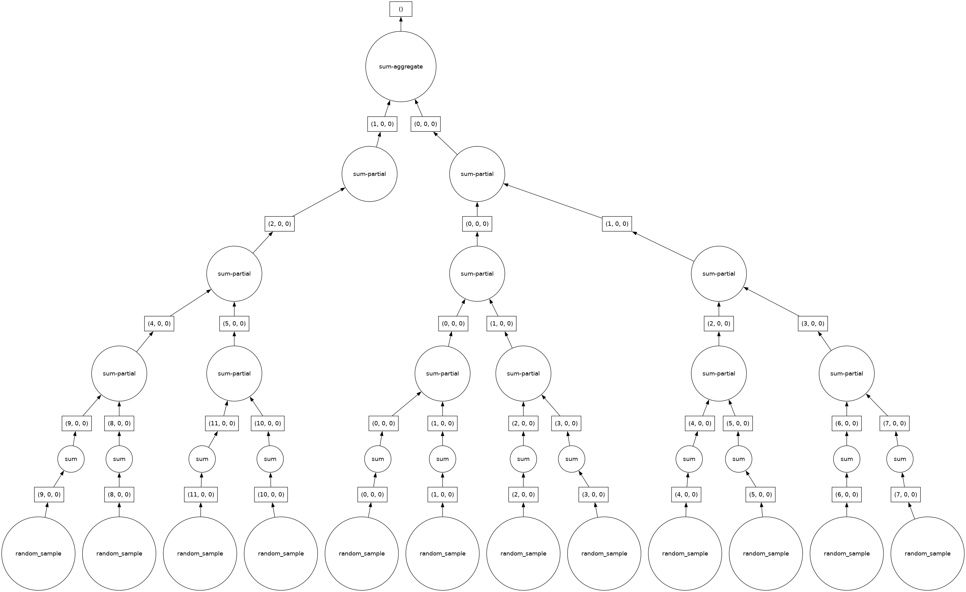
As is obvious from the above exercise, Dask quickly and easily determines a strategy for performing the operations, in this case a sum. This illustrates the appeal of Dask: automatic algorithm generation that scales from simple arithmetic problems to highly complex scientific equations with large datasets and multiple operations.
In this next set of examples, we demonstrate that increasing the complexity of the operations performed also increases the complexity of the Dask graph.
In this example, we use randomly selected functions, arguments and Python slices to create a complex set of operations. We then visualize the Dask graph to illustrate the increased complexity:
z = darr.dot(darr.T).mean(axis=0)[::2, :].std(axis=1)
zz.visualize()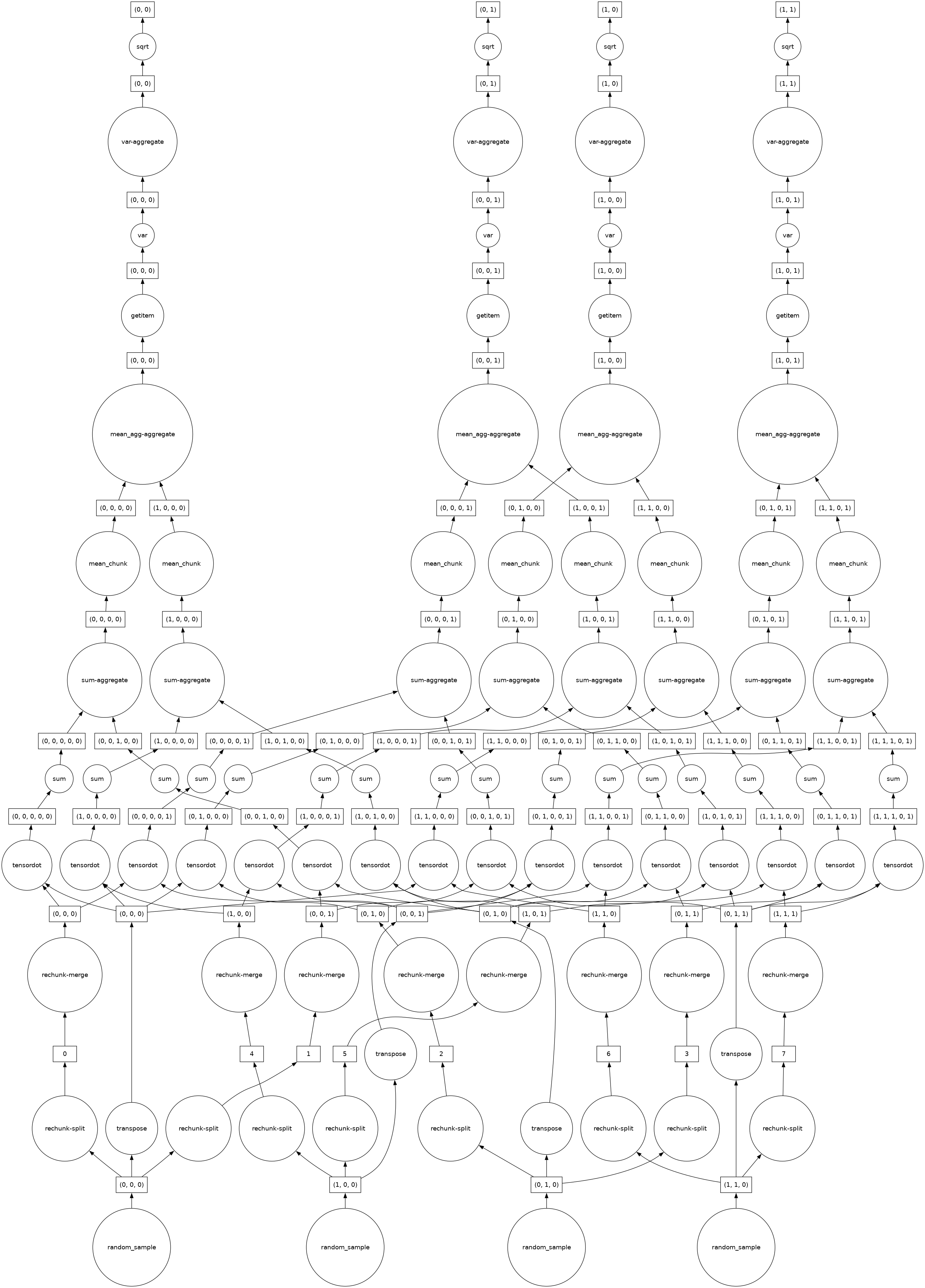
Testing a bigger calculation
While the earlier examples in this tutorial described well the basics of Dask, the size of the data in those examples, about 180 MB, is far too small for an actual use of Dask.
In this example, we create a much larger array, more indicative of data actually used in Dask:
darr = da.random.random((4000, 100, 4000), chunks=(1000, 100, 500)).astype('float32')
darrThe dataset created in the previous example is much larger, approximately 6 GB. Depending on how many programs are running on your computer, this may be greater than the amount of free RAM on your computer. However, as Dask is larger-than-memory, the amount of free RAM does not impede Dask’s ability to work on this dataset.
In this example, we again perform randomly selected operations, but this time on the much larger dataset. We also visualize the Dask graph, and then run the compute method. However, as computing complex functions on large datasets is inherently time-consuming, we show a progress bar to track the progress of the computation.
z = (darr + darr.T)[::2, :].mean(axis=2)z.visualize()
with ProgressBar():
    computed_ds = z.compute()
[ ] | 0% Completed | 361.93 us[ ] | 0% Completed | 109.32 ms[ ] | 0% Completed | 215.55 ms[ ] | 0% Completed | 316.35 ms[ ] | 0% Completed | 417.10 ms[ ] | 0% Completed | 517.77 ms[ ] | 0% Completed | 618.40 ms[ ] | 1% Completed | 719.16 ms[# ] | 2% Completed | 825.42 ms[## ] | 5% Completed | 926.30 ms[### ] | 8% Completed | 1.03 s[#### ] | 10% Completed | 1.13 s[#### ] | 10% Completed | 1.23 s[#### ] | 10% Completed | 1.33 s[#### ] | 10% Completed | 1.43 s[#### ] | 10% Completed | 1.53 s[#### ] | 10% Completed | 1.64 s[#### ] | 10% Completed | 1.74 s[#### ] | 11% Completed | 1.84 s[##### ] | 12% Completed | 1.94 s[##### ] | 14% Completed | 2.04 s[###### ] | 17% Completed | 2.15 s[####### ] | 19% Completed | 2.25 s[######## ] | 21% Completed | 2.35 s[######## ] | 22% Completed | 2.45 s[######## ] | 22% Completed | 2.55 s[######## ] | 22% Completed | 2.65 s[######## ] | 22% Completed | 2.76 s[######## ] | 22% Completed | 2.86 s[######### ] | 22% Completed | 2.96 s[######### ] | 23% Completed | 3.06 s[########## ] | 25% Completed | 3.17 s[########### ] | 28% Completed | 3.27 s[############ ] | 31% Completed | 3.37 s[############# ] | 33% Completed | 3.48 s[############# ] | 34% Completed | 3.58 s[############# ] | 34% Completed | 3.68 s[############# ] | 34% Completed | 3.78 s[############# ] | 34% Completed | 3.89 s[############# ] | 34% Completed | 3.99 s[############# ] | 34% Completed | 4.09 s[############# ] | 34% Completed | 4.19 s[############## ] | 36% Completed | 4.29 s[############### ] | 38% Completed | 4.39 s[################ ] | 40% Completed | 4.49 s[################# ] | 42% Completed | 4.60 s[################## ] | 45% Completed | 4.70 s[################### ] | 47% Completed | 4.81 s[################### ] | 47% Completed | 4.91 s[################### ] | 47% Completed | 5.01 s[################### ] | 47% Completed | 5.11 s[################### ] | 47% Completed | 5.21 s[################### ] | 47% Completed | 5.31 s[################### ] | 48% Completed | 5.41 s[################### ] | 49% Completed | 5.52 s[#################### ] | 51% Completed | 5.62 s[##################### ] | 53% Completed | 5.72 s[###################### ] | 55% Completed | 5.82 s[####################### ] | 59% Completed | 5.93 s[####################### ] | 59% Completed | 6.03 s[####################### ] | 59% Completed | 6.13 s[####################### ] | 59% Completed | 6.23 s[####################### ] | 59% Completed | 6.33 s[####################### ] | 59% Completed | 6.43 s[####################### ] | 59% Completed | 6.54 s[####################### ] | 59% Completed | 6.64 s[######################## ] | 60% Completed | 6.74 s[######################### ] | 62% Completed | 6.84 s[########################## ] | 65% Completed | 6.94 s[########################### ] | 68% Completed | 7.05 s[############################ ] | 71% Completed | 7.15 s[############################# ] | 74% Completed | 7.25 s[############################# ] | 74% Completed | 7.35 s[############################# ] | 74% Completed | 7.45 s[############################# ] | 74% Completed | 7.55 s[############################# ] | 74% Completed | 7.66 s[############################# ] | 74% Completed | 7.76 s[############################# ] | 74% Completed | 7.86 s[############################## ] | 75% Completed | 7.96 s[############################## ] | 76% Completed | 8.06 s[############################### ] | 78% Completed | 8.16 s[################################ ] | 80% Completed | 8.26 s[################################# ] | 83% Completed | 8.37 s[################################## ] | 85% Completed | 8.47 s[################################## ] | 85% Completed | 8.57 s[################################## ] | 85% Completed | 8.67 s[################################## ] | 85% Completed | 8.78 s[################################## ] | 85% Completed | 8.88 s[################################## ] | 85% Completed | 8.98 s[################################## ] | 85% Completed | 9.09 s[################################## ] | 86% Completed | 9.19 s[################################### ] | 87% Completed | 9.29 s[################################### ] | 89% Completed | 9.39 s[#################################### ] | 92% Completed | 9.49 s[###################################### ] | 95% Completed | 9.60 s[###################################### ] | 97% Completed | 9.70 s[########################################] | 100% Completed | 9.80 s
Dask Arrays with Xarray
While directly interacting with Dask Arrays can be useful on occasion, more often than not Dask Arrays are interacted with through Xarray. Since Xarray wraps NumPy arrays, and Dask Arrays contain most of the functionality of NumPy arrays, Xarray can also wrap Dask Arrays, allowing anyone with knowledge of Xarray to easily start using the Dask interface.
Reading data with Dask and Xarray
As demonstrated in previous examples, a Dask Array consists of many smaller arrays, called chunks:
darrAs shown in the following example, to read data into Xarray as Dask Arrays, simply specify the chunks keyword argument when calling the open_dataset() function:
ds = xr.open_dataset(DATASETS.fetch('CESM2_sst_data.nc'), chunks={})
ds.tosWhile it is a valid operation to pass an empty list to the chunks keyword argument, this technique does not specify how to chunk the data, and therefore the resulting Dask Array contains only one chunk.
Correct usage of the chunks keyword argument specifies how many values in each dimension are contained in a single chunk. In this example, specifying the chunks keyword argument as chunks={'time':90} indicates to Xarray and Dask that 90 time slices are allocated to each chunk on the temporal axis.
Since this dataset contains 180 total time slices, the data variable tos (holding the sea surface temperature data) is now split into two chunks in the temporal dimension.
ds = xr.open_dataset(
    DATASETS.fetch('CESM2_sst_data.nc'),
    engine="netcdf4",
    chunks={"time": 90, "lat": 180, "lon": 360},
)
ds.tosIt is fairly straightforward to retrieve a list of the chunks and their sizes for each dimension; simply call the .chunks method on an Xarray DataArray. In this example, we show that the tos DataArray now contains two chunks on the time dimension, with each chunk containing 90 time slices.
ds.tos.chunks((90, 90), (180,), (360,))Xarray data structures are first-class dask collections
If an Xarray Dataset or DataArray object uses a Dask Array, rather than a NumPy array, it counts as a first-class Dask collection. This means that you can pass such an object to dask.visualize() and dask.compute(), in the same way as an individual Dask Array.
In this example, we call dask.visualize on our Xarray DataArray, displaying a Dask graph for the DataArray object:
dask.visualize(ds)
Parallel and lazy computation using dask.array with Xarray
As described above, Xarray Datasets and DataArrays containing Dask Arrays are first-class Dask collections. Therefore, computations performed on such objects are deferred until a compute method is called. (This is the definition of lazy computation.)
z = ds.tos.mean(['lat', 'lon']).dot(ds.tos.T)
zAs shown in the above example, the result of the applied operations is an Xarray DataArray that contains a Dask Array, an identical object type to the object that the operations were performed on. This is true for any operations that can be applied to Xarray DataArrays, including subsetting operations; this next example illustrates this:
z.isel(lat=0)Because the data subset created above is also a first-class Dask collection, we can view its Dask graph using the dask.visualize() function, as shown in this example:
dask.visualize(z)
Since this object is a first-class Dask collection, the computations performed on it have been deferred. To run these computations, we must call a compute method, in this case .compute(). This example also uses a progress bar to track the computation progress.
with ProgressBar():
    computed_ds = z.compute()
[ ] | 0% Completed | 268.01 us[#################################### ] | 90% Completed | 102.15 ms[########################################] | 100% Completed | 203.15 ms
Summary
This tutorial covered the use of Xarray to access Dask Arrays, and the use of the chunks keyword argument to open datasets with Dask data instead of NumPy data. Another important concept introduced in this tutorial is the usage of Xarray Datasets and DataArrays as Dask collections, allowing Xarray objects to be manipulated in a similar manner to Dask Arrays. Finally, the concepts of larger-than-memory datasets, lazy computation, and parallel computation, and how they relate to Xarray and Dask, were covered.
Dask Shortcomings
Although Dask Arrays and NumPy arrays are generally interchangeable, NumPy offers some functionality that is lacking in Dask Arrays. The usage of Dask Array comes with the following relevant issues:
- Operations where the resulting shape depends on the array values can produce erratic behavior, or fail altogether, when used on a Dask Array. If the operation succeeds, the resulting Dask Array will have unknown chunk sizes, which can cause other sections of code to fail.
- Operations that are by nature difficult to parallelize or less useful on very large datasets, such as
sort, are not included in the Dask Array interface. Some of these operations have supported versions that are inherently more intuitive to parallelize, such astopk. - Development of new Dask functionality is only initiated when such functionality is required; therefore, some lesser-used NumPy functions, such as
np.sometrue, are not yet implemented in Dask. However, many of these functions can be added as community contributions, or have already been added in this manner.
Learn More
For more in-depth information on Dask Arrays, visit the official documentation page. In addition, this screencast reinforces the concepts covered in this tutorial. (If you are viewing this page as a Jupyter Notebook, the screencast will appear below as an embedded YouTube video.)
from IPython.display import YouTubeVideo

YouTubeVideo(id="9h_61hXCDuI", width=600, height=300)Resources and references
To find specific reference information about Dask and Xarray, see the official documentation pages listed below:
If you require assistance with a specific issue involving Xarray or Dask, the following resources may be of use:
- Dask tag on StackOverflow, for usage questions
- github discussions: dask for general, non-bug, discussion, and usage questions
- github issues: dask for bug reports and feature requests
- github discussions: xarray for general, non-bug, discussion, and usage questions
- github issues: xarray for bug reports and feature requests
Certain sections of this tutorial are adapted from the following existing tutorials: